
set.seed(8)
#The number of samples
n.x <- 20
#Create x values that at uniformly distributed throughout the rate of 1 to 20
x <- sort(runif(n = n.x, min = 1, max =20))
mm <- model.matrix(~x)
intercept <- 0.6
slope=0.1
#The linear predictor
linpred <- mm %*% c(intercept,slope)
#Predicted y values
lambda <- exp(linpred)
#Add some noise and make binomial
y <- rpois(n=n.x, lambda=lambda)
dat <- data.frame(y,x)Generalised Linear Models part II (JAGS)
Quarto
R
Academia
Software
Statistics
Abstract
The focus of this simple tutorial is to provide a brief introduction and overview about how to fit Bayesian models using JAGS via R …
Keywords
Software, Statistics, Stan
This tutorial will focus on the use of Bayesian estimation to fit simple linear regression models. BUGS (Bayesian inference Using Gibbs Sampling) is an algorithm and supporting language (resembling R) dedicated to performing the Gibbs sampling implementation of Markov Chain Monte Carlo (MCMC) method. Dialects of the BUGS language are implemented within three main projects:
OpenBUGS - written in component pascal.
JAGS - (Just Another Gibbs Sampler) - written in
C++.STAN - a dedicated Bayesian modelling framework written in
C++and implementing Hamiltonian MCMC samplers.
Whilst the above programs can be used stand-alone, they do offer the rich data pre-processing and graphical capabilities of R, and thus, they are best accessed from within R itself. As such there are multiple packages devoted to interfacing with the various software implementations:
R2OpenBUGS - interfaces with
OpenBUGSR2jags - interfaces with
JAGSrstan - interfaces with
STAN
This tutorial will demonstrate how to fit models in JAGS (Plummer (2004)) using the package R2jags (Su et al. (2015)) as interface, which also requires to load some other packages.
Overview
Introduction
Whilst in many instances, count data can be approximated reasonably well by a normal distribution (particularly if the counts are all above zero and the mean count is greater than about \(20\)), more typically, when count data are modelled via normal distribution certain undesirable characteristics arise that are a consequence of the nature of discrete non-negative data.
Expected (predicted) values and confidence bands less than zero are illogical, yet these are entirely possible from a normal distribution
The distribution of count data are often skewed when their mean is low (in part because the distribution is truncated to the left by zero) and variance usually increases with increasing mean (variance is typically proportional to mean in count data). By contrast, the Gaussian (normal) distribution assumes that mean and variance are unrelated and thus estimates (particularly of standard error) might well be reasonable inaccurate.
Poisson regression is a type of generalised linear model (GLM) in which a non-negative integer (natural number) response is modelled against a linear predictor via a specific link function. The linear predictor is typically a linear combination of effects parameters. The role of the link function is to transform the expected values of the response y (which is on the scale of (\(0;\infty\)), as is the Poisson distribution from which expectations are drawn) into the scale of the linear predictor (which is \(-\infty;\infty\)).
As implied in the name of this group of analyses, a Poisson rather than Gaussian (normal) distribution is used to represent the errors (residuals). Like count data (number of individuals, species etc), the Poisson distribution encapsulates positive integers and is bound by zero at one end. Consequently, the degree of variability is directly related the expected value (equivalent to the mean of a Gaussian distribution). Put differently, the variance is a function of the mean. Repeated observations from a Poisson distribution located close to zero will yield a much smaller spread of observations than will samples drawn from a Poisson distribution located a greater distance from zero. In the Poisson distribution, the variance has a 1:1 relationship with the mean. The canonical link function for the Poisson distribution is a log-link function.
Whilst the expectation that the mean=variance (\(\mu=\sigma\)) is broadly compatible with actual count data (that variance increases at the same rate as the mean), under certain circumstances, this might not be the case. For example, when there are other unmeasured influences on the response variable, the distribution of counts might be somewhat clumped which can result in higher than expected variability (that is \(\sigma > \mu\)). The variance increases more rapidly than does the mean. This is referred to as overdispersion. The degree to which the variability is greater than the mean (and thus the expected degree of variability) is called dispersion. Effectively, the Poisson distribution has a dispersion parameter (or scaling factor) of \(1\).
It turns out that overdispersion is very common for count data and it typically underestimates variability, standard errors and thus deflated p-values. There are a number of ways of overcoming this limitation, the effectiveness of which depend on the causes of overdispersion.
Quasi-Poisson models - these introduce the dispersion parameter (\(\phi\)) into the model. This approach does not utilize an underlying error distribution to calculate the maximum likelihood (there is no quasi-Poisson distribution). Instead, if the Newton-Ralphson iterative reweighting least squares algorithm is applied using a direct specification of the relationship between mean and variance (\(\text{var}(y)=\phi\mu\), the estimates of the regression coefficients are identical to those of the maximum likelihood estimates from the Poisson model. This is analogous to fitting ordinary least squares on symmetrical, yet not normally distributed data - the parameter estimates are the same, however they won’t necessarily be as efficient. The standard errors of the coefficients are then calculated by multiplying the Poisson model coefficient standard errors by \(\sqrt{\phi}\). Unfortunately, because the quasi-poisson model is not estimated via maximum likelihood, properties such as AIC and log-likelihood cannot be derived. Consequently, quasi-poisson and Poisson model fits cannot be compared via either AIC or likelihood ratio tests (nor can they be compared via deviance as uasi-poisson and Poisson models have the same residual deviance). That said, quasi-likelihood can be obtained by dividing the likelihood from the Poisson model by the dispersion (scale) factor.
Negative binomial model - technically, the negative binomial distribution is a probability distribution for the number of successes before a specified number of failures. However, the negative binomial can also be defined (parameterised) in terms of a mean (\(\mu\)) and scale factor (\(\omega\)),
\[ p(y_i) = \frac{\Gamma(y_i+\omega)}{\Gamma(\omega)y!} \times \frac{\mu^{y_i}_i\omega^\omega}{(\mu_i+\omega)^{\mu_i+\omega}}, \]
where the expectected value of the values \(y_i\) (the means) are (\(\mu_i\)) and the variance is \(y_i=\frac{\mu_i+\mu^2_i}{\omega}\). In this way, the negative binomial is a two-stage hierarchical process in which the response is modeled against a Poisson distribution whose expected count is in turn modeled by a Gamma distribution with a mean of \(\mu\) and constant scale parameter (\(\omega\)). Strictly, the negative binomial is not an exponential family distribution (unless \(\omega\) is fixed as a constant), and thus negative binomial models cannot be fit via the usual GLM iterative reweighting algorithm. Instead estimates of the regression parameters along with the scale factor (\(\omega\)) are obtained via maximum likelihood. The negative binomial model is useful for accommodating overdispersal when it is likely caused by clumping (due to the influence of other unmeasured factors) within the response.
Zero-inflated Poisson model - overdispersion can also be caused by the presence of a greater number of zero’s than would otherwise be expected for a Poisson distribution. There are potentially two sources of zero counts - genuine zeros and false zeros. Firstly, there may genuinely be no individuals present. This would be the number expected by a Poisson distribution. Secondly, individuals may have been present yet not detected or may not even been possible. These are false zero’s and lead to zero inflated data (data with more zeros than expected). For example, the number of joeys accompanying an adult koala could be zero because the koala has no offspring (true zero) or because the koala is male or infertile (both of which would be examples of false zeros). Similarly, zero counts of the number of individual in a transect are due either to the absence of individuals or the inability of the observer to detect them. Whilst in the former example, the latent variable representing false zeros (sex or infertility) can be identified and those individuals removed prior to analysis, this is not the case for the latter example. That is, we cannot easily partition which counts of zero are due to detection issues and which are a true indication of the natural state.
Consistent with these two sources of zeros, zero-inflated models combine a binary logistic regression model (that models count membership according to a latent variable representing observations that can only be zeros - not detectable or male koalas) with a Poisson regression (that models count membership according to a latent variable representing observations whose values could be 0 or any positive integer - fertile female koalas).
Poisson regression
The following equations are provided since in Bayesian modelling, it is occasionally necessary to directly define the log-likelihood calculations (particularly for zero-inflated models and other mixture models).
\[ f(y \mid \lambda) = \frac{\lambda^ye^{-\lambda}}{y!}, \]
where \(E[Y]=Var(Y)=\lambda\) and \(\lambda\) is the mean.
Data generation
Lets say we wanted to model the abundance of an item (\(y\)) against a continuous predictor (\(x\)). As this section is mainly about the generation of artificial data (and not specifically about what to do with the data), understanding the actual details are optional and can be safely skipped.
With these sort of data, we are primarily interested in investigating whether there is a relationship between the binary response variable and the linear predictor (linear combination of one or more continuous or categorical predictors).
Exploratory data analysis
There are at least five main potential models we could consider fitting to these data:
Ordinary least squares regression (general linear model) - assumes normality of residuals
Poisson regression - assumes mean=variance (dispersion\(=1\))
Quasi-poisson regression - a general solution to overdispersion. Assumes variance is a function of mean, dispersion estimated, however likelihood based statistics unavailable
Negative binomial regression - a specific solution to overdispersion caused by clumping (due to an unmeasured latent variable). Scaling factor (\(\omega\)) is estimated along with the regression parameters.
Zero-inflation model - a specific solution to overdispersion caused by excessive zeros (due to an unmeasured latent variable). Mixture of binomial and Poisson models.
When counts are all very large (not close to \(0\)) and their ranges do not span orders of magnitude, they take on very Gaussian properties (symmetrical distribution and variance independent of the mean). Given that models based on the Gaussian distribution are more optimized and recognized than Generalized Linear Models, it can be prudent to adopt Gaussian models for such data. Hence it is a good idea to first explore whether a Poisson model is likely to be more appropriate than a standard Gaussian model. The potential for overdispersion can be explored by adding a rug to boxplot. The rug is simply tick marks on the inside of an axis at the position corresponding to an observation. As multiple identical values result in tick marks drawn over one another, it is typically a good idea to apply a slight amount of jitter (random displacement) to the values used by the rug.
hist(dat$x)
boxplot(dat$y, horizontal=TRUE)
rug(jitter(dat$y), side=1)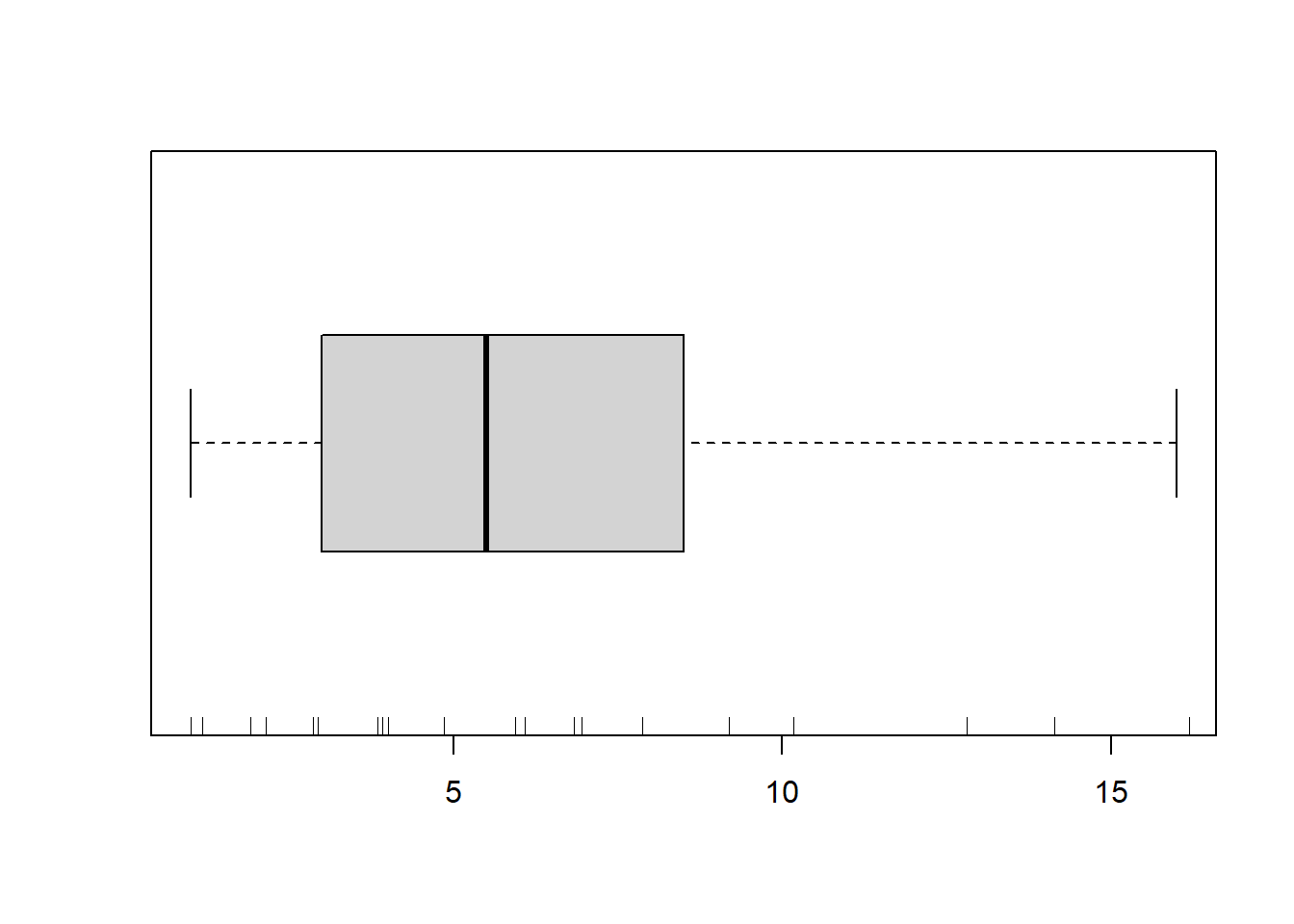
There is definitely signs of non-normality that would warrant Poisson models. The rug applied to the boxplots does not indicate a series degree of clumping and there appears to be few zero. Thus overdispersion is unlikely to be an issue. Lets now explore linearity by creating a histogram of the predictor variable (\(x\)) and a scatterplot of the relationship between the response (\(y\)) and the predictor (\(x\))
#now for the scatterplot
plot(y~x, dat, log="y")
with(dat, lines(lowess(y~x)))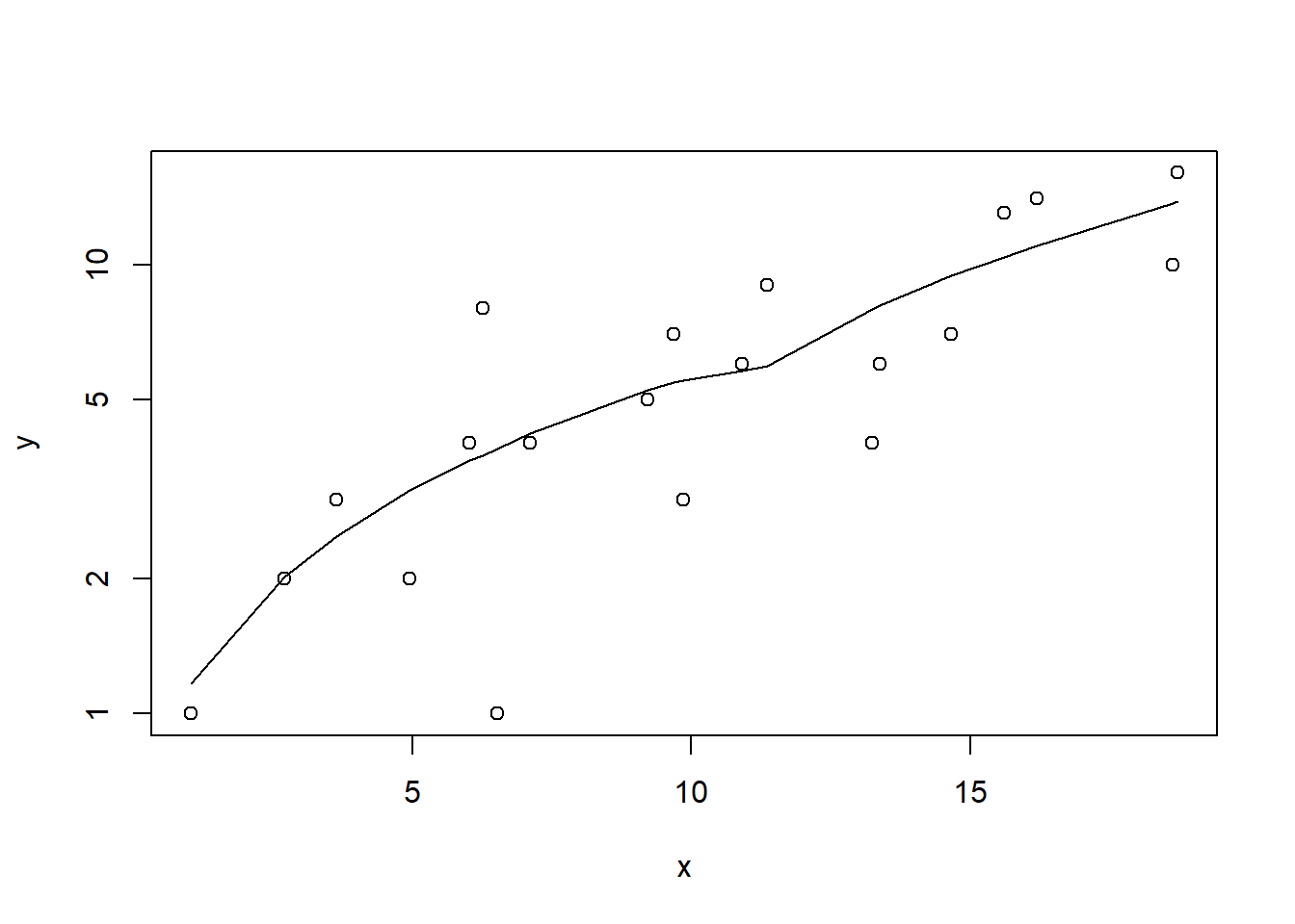
Conclusions: the predictor (\(x\)) does not display any skewness or other issues that might lead to non-linearity. The lowess smoother on the scatterplot does not display major deviations from a straight line and thus linearity is satisfied. Violations of linearity could be addressed by either:
define a non-linear linear predictor (such as a polynomial, spline or other non-linear function).
transform the scale of the predictor variables.
Although we have already established that there are few zeros in the data (and thus overdispersion is unlikely to be an issue), we can also explore this by comparing the number of zeros in the data to the number of zeros that would be expected from a Poisson distribution with a mean equal to the mean count of the data.
#proportion of 0's in the data
dat.tab<-table(dat$y==0)
dat.tab/sum(dat.tab)
NA
NA FALSE
NA 1#proportion of 0's expected from a Poisson distribution
mu <- mean(dat$y)
cnts <- rpois(1000, mu)
dat.tab <- table(cnts == 0)
dat.tab/sum(dat.tab)NA
NA FALSE TRUE
NA 0.997 0.003In the above, the value under FALSE is the proportion of non-zero values in the data and the value under TRUE is the proportion of zeros in the data. In this example, there are no zeros in the observed data which corresponds closely to the very low proportion expected (\(0.003\)).
Model fitting
\[ y_i \sim \text{Pois}(\lambda_i), \]
where \(\log(\lambda_i)=\eta_i\), with \(\eta_i=\beta_0+\beta_1x_{i}\) and \(\beta_0,\beta_1 \sim N(0, 10000)\).
dat.list <- with(dat,list(Y=y, X=x,N=nrow(dat)))
modelString="
model {
  for (i in 1:N) {
     Y[i] ~ dpois(lambda[i])
     log(lambda[i]) <- beta0 + beta1*X[i]
  }
  beta0 ~ dnorm(0,1.0E-06)
  beta1 ~ dnorm(0,1.0E-06)
}
"
writeLines(modelString, con='modelpois.txt')

params <- c('beta0','beta1')
nChains = 2
burnInSteps = 5000
thinSteps = 1
numSavedSteps = 20000
nIter = ceiling((numSavedSteps * thinSteps)/nChains)

library(R2jags)
dat.P.jags <- jags(data=dat.list,model.file='modelpois.txt', param=params,
                   n.chains=nChains, n.iter=nIter, n.burnin=burnInSteps, n.thin=thinSteps)
NA Compiling model graph
NA Resolving undeclared variables
NA Allocating nodes
NA Graph information:
NA Observed stochastic nodes: 20
NA Unobserved stochastic nodes: 2
NA Total graph size: 105
NA
NA Initializing modelModel evaluation
library(mcmcplots)
denplot(dat.P.jags, parms = c("beta0","beta1"))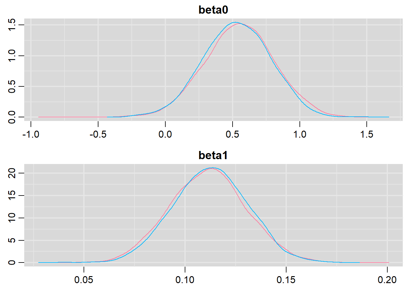
traplot(dat.P.jags, parms = c("beta0","beta1"))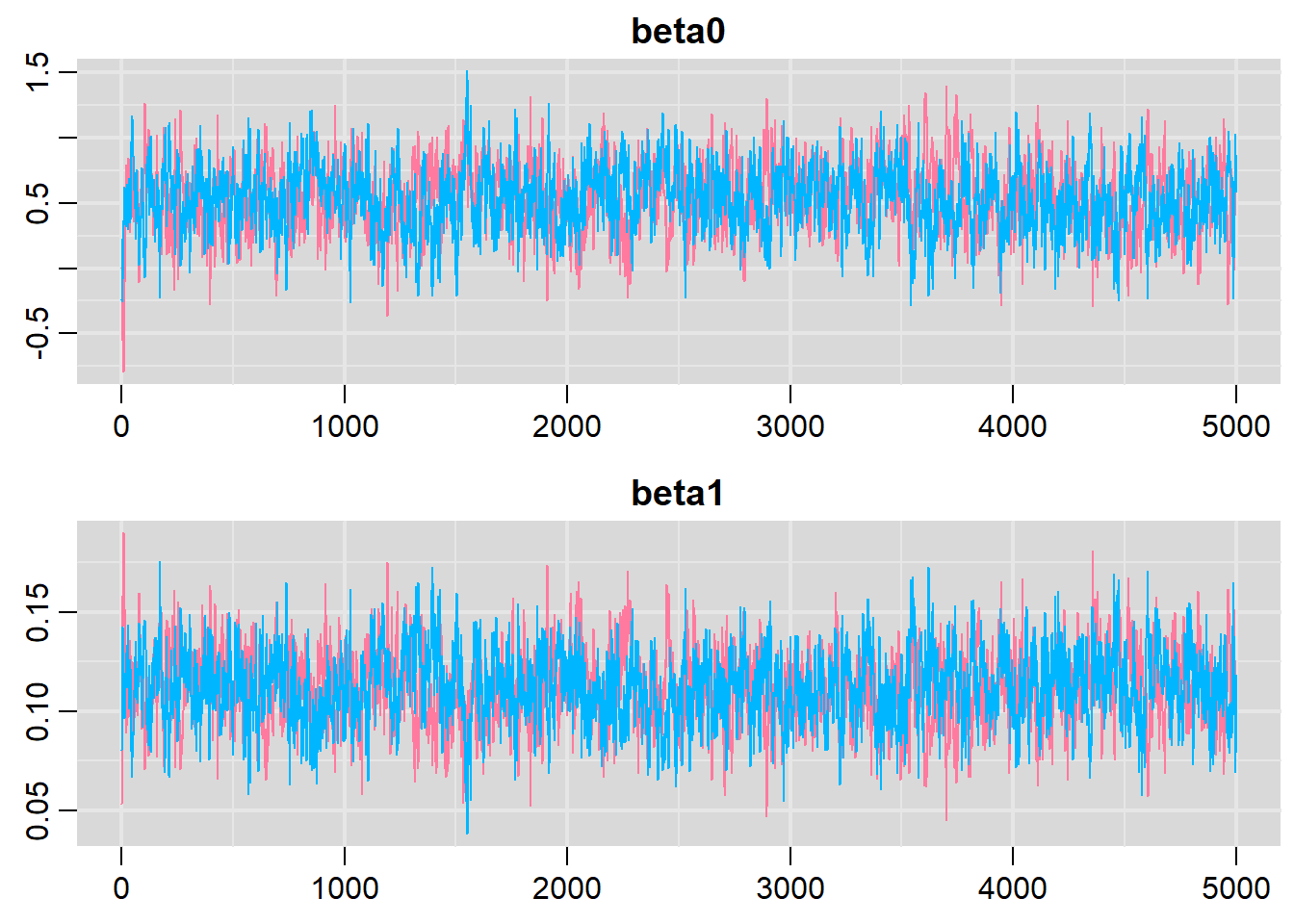
raftery.diag(as.mcmc(dat.P.jags))NA [[1]]
NA
NA Quantile (q) = 0.025
NA Accuracy (r) = +/- 0.005
NA Probability (s) = 0.95
NA
NA Burn-in Total Lower bound Dependence
NA (M) (N) (Nmin) factor (I)
NA beta0 10 10830 3746 2.89
NA beta1 12 12612 3746 3.37
NA deviance 3 4410 3746 1.18
NA
NA
NA [[2]]
NA
NA Quantile (q) = 0.025
NA Accuracy (r) = +/- 0.005
NA Probability (s) = 0.95
NA
NA Burn-in Total Lower bound Dependence
NA (M) (N) (Nmin) factor (I)
NA beta0 12 14878 3746 3.97
NA beta1 10 11942 3746 3.19
NA deviance 2 3995 3746 1.07autocorr.diag(as.mcmc(dat.P.jags))NA beta0 beta1 deviance
NA Lag 0 1.00000000 1.0000000000 1.000000000
NA Lag 1 0.83977964 0.8111423616 0.508803232
NA Lag 5 0.43884918 0.3859514845 0.118732714
NA Lag 10 0.22584100 0.1883831873 0.029775648
NA Lag 50 -0.01164622 -0.0003926876 -0.007507996One very important model validation procedure is to examine a plot of residuals against predicted or fitted values (the residual plot). Ideally, residual plots should show a random scatter of points without outliers. That is, there should be no patterns in the residuals. Patterns suggest inappropriate linear predictor (or scale) and/or inappropriate residual distribution/link function. The residuals used in such plots should be standardized (particularly if the model incorporated any variance-covariance structures - such as an autoregressive correlation structure) Pearsons’s residuals standardize residuals by division with the square-root of the variance. We can generate Pearson’s residuals within the JAGS model. Alternatively, we could use the parameters to generate the residuals outside of JAGS. Pearson’s residuals are calculated according to:
\[ \epsilon = \frac{y_i - \mu}{\sqrt{\text{var}(y)}}, \]
where \(\mu\) is the expected value of \(Y\) (\(=\lambda\) for Poisson) and var(\(y\)) is the variance of \(Y\) (\(=\lambda\) for Poisson).
#extract the samples for the two model parameters
coefs <- dat.P.jags$BUGSoutput$sims.matrix[,1:2]
Xmat <- model.matrix(~x, data=dat)
#expected values on a log scale
eta<-coefs %*% t(Xmat)
#expected value on response scale
lambda <- exp(eta)
#Expected value and variance are both equal to lambda
expY <- varY <- lambda
#sweep across rows and then divide by lambda
Resid <- -1*sweep(expY,2,dat$y,'-')/sqrt(varY)
#plot residuals vs expected values
plot(apply(Resid,2,mean)~apply(eta,2,mean))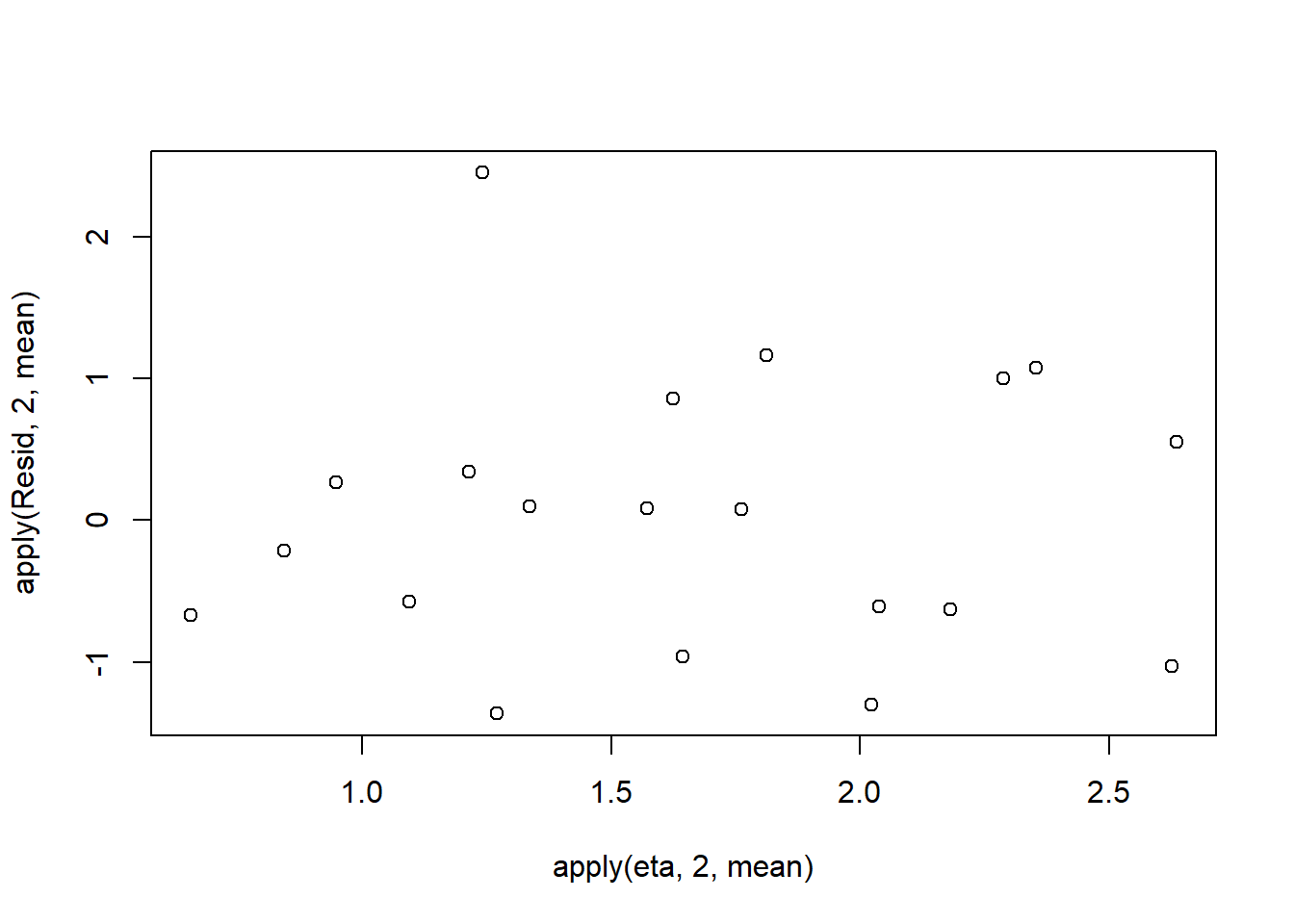
Now we will compare the sum of squared residuals to the sum of squares residuals that would be expected from a Poisson distribution matching that estimated by the model. Essentially this is estimating how well the Poisson distribution, the log-link function and the linear model approximates the observed data.
SSres<-apply(Resid^2,1,sum)

#generate a matrix of draws from a poisson distribution
# the matrix is the same dimensions as lambda and uses the probabilities of lambda
YNew <- matrix(rpois(length(lambda),lambda=lambda),nrow=nrow(lambda))

Resid1<-(lambda - YNew)/sqrt(lambda)
SSres.sim<-apply(Resid1^2,1,sum)
mean(SSres.sim>SSres, na.rm = T)
NA [1] 0.4697Goodness of fit
dat.list1 <- with(dat,list(Y=y, X=x,N=nrow(dat)))
modelString="
model {
  for (i in 1:N) {
    #likelihood function
    Y[i] ~ dpois(lambda[i])
    eta[i] <- beta0+beta1*X[i] #linear predictor
    log(lambda[i]) <- eta[i]   #link function

    #E(Y) and var(Y)
    expY[i] <- lambda[i]
    varY[i] <- lambda[i]

    # Calculate RSS
    Resid[i] <- (Y[i] - expY[i])/sqrt(varY[i])
    RSS[i] <- pow(Resid[i],2)

    #Simulate data from a Poisson distribution
    Y1[i] ~ dpois(lambda[i])
    #Calculate RSS for simulated data
    Resid1[i] <- (Y1[i] - expY[i])/sqrt(varY[i])
    RSS1[i] <-pow(Resid1[i],2)
  }
  #Priors
  beta0 ~ dnorm(0,1.0E-06)
  beta1 ~ dnorm(0,1.0E-06)
  #Bayesian P-value
  Pvalue <- mean(sum(RSS1)>sum(RSS))
}
"

writeLines(modelString, con='modelpois_gof.txt')

params <- c('beta0','beta1', 'Pvalue')
nChains = 2
burnInSteps = 5000
thinSteps = 1
numSavedSteps = 20000
nIter = ceiling((numSavedSteps * thinSteps)/nChains)

dat.P.jags1 <- jags(data=dat.list,model.file='modelpois_gof.txt', param=params,
                   n.chains=nChains, n.iter=nIter, n.burnin=burnInSteps, n.thin=thinSteps)
NA Compiling model graph
NA Resolving undeclared variables
NA Allocating nodes
NA Graph information:
NA Observed stochastic nodes: 20
NA Unobserved stochastic nodes: 22
NA Total graph size: 272
NA
NA Initializing modelprint(dat.P.jags1)NA Inference for Bugs model at "modelpois_gof.txt", fit using jags,
NA 2 chains, each with 10000 iterations (first 5000 discarded)
NA n.sims = 10000 iterations saved
NA mu.vect sd.vect 2.5% 25% 50% 75% 97.5% Rhat n.eff
NA Pvalue 0.478 0.500 0.000 0.000 0.000 1.000 1.000 1.001 10000
NA beta0 0.546 0.254 0.015 0.381 0.559 0.719 1.013 1.001 10000
NA beta1 0.112 0.018 0.077 0.099 0.111 0.124 0.149 1.001 3200
NA deviance 88.372 3.041 86.373 86.883 87.671 89.075 93.868 1.006 2000
NA
NA For each parameter, n.eff is a crude measure of effective sample size,
NA and Rhat is the potential scale reduction factor (at convergence, Rhat=1).
NA
NA DIC info (using the rule, pD = var(deviance)/2)
NA pD = 4.6 and DIC = 93.0
NA DIC is an estimate of expected predictive error (lower deviance is better).Conclusions: the Bayesian p-value is approximately \(0.5\), suggesting that there is a good fit of the model to the data.
Unfortunately, unlike with linear models (Gaussian family), the expected distribution of data (residuals) varies over the range of fitted values for numerous (often competing) ways that make diagnosing (and attributing causes thereof) miss-specified generalized linear models from standard residual plots very difficult. The use of standardized (Pearson) residuals or deviance residuals can partly address this issue, yet they still do not offer completely consistent diagnoses across all issues (miss-specified model, over-dispersion, zero-inflation). An alternative approach is to use simulated data from the model posteriors to calculate an empirical cumulative density function from which residuals are are generated as values corresponding to the observed data along the density function. Now we will compare the sum of squared residuals to the sum of squares residuals that would be expected from a Bernoulli distribution matching that estimated by the model. Essentially this is estimating how well the Bernoulli distribution and linear model approximates the observed data.
#extract the samples for the two model parameters
coefs <- dat.P.jags$BUGSoutput$sims.matrix[,1:2]
Xmat <- model.matrix(~x, data=dat)
#expected values on a log scale
eta<-coefs %*% t(Xmat)
#expected value on response scale
lambda <- exp(eta)

simRes <- function(lambda, data,n=250, plot=T, family='poisson') {
 require(gap)
 N = nrow(data)
 sim = switch(family,
    'poisson' = matrix(rpois(n*N,apply(lambda,2,mean)),ncol=N, byrow=TRUE)
 )
 a = apply(sim + runif(n,-0.5,0.5),2,ecdf)
 resid<-NULL
 for (i in 1:nrow(data)) resid<-c(resid,a[[i]](data$y[i] + runif(1 ,-0.5,0.5)))
 if (plot==T) {
   par(mfrow=c(1,2))
   gap::qqunif(resid,pch = 2, bty = "n",
   logscale = F, col = "black", cex = 0.6, main = "QQ plot residuals",
   cex.main = 1, las=1)
   plot(resid~apply(lambda,2,mean), xlab='Predicted value', ylab='Standardized residual', las=1)
 }
 resid
}

simRes(lambda,dat, family='poisson')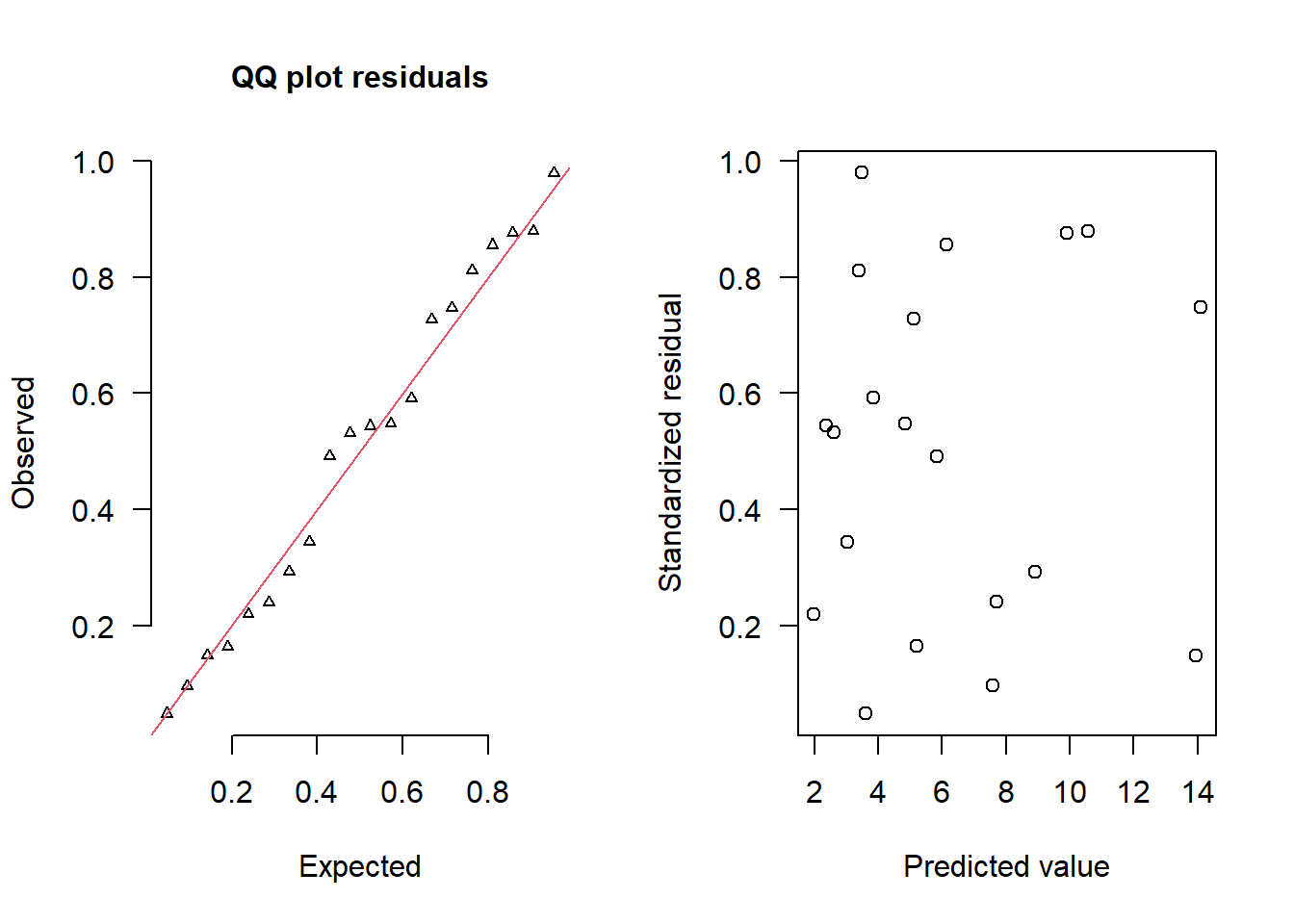
NA  [1] 0.220 0.544 0.532 0.344 0.812 0.980 0.048 0.592 0.548 0.728 0.164 0.492
NA [13] 0.856 0.096 0.240 0.292 0.876 0.880 0.148 0.748
The trend (black symbols) in the qq-plot does not appear to be overly non-linear (matching the ideal red line well), suggesting that the model is not overdispersed. The spread of standardized (simulated) residuals in the residual plot do not appear overly non-uniform. That is there is not trend in the residuals. Furthermore, there is not a concentration of points close to \(1\) or \(0\) (which would imply overdispersion).
Recall that the Poisson regression model assumes that variance=mean (var=μϕ where \(\phi=1\)) and thus dispersion (\(\phi=\frac{\text{var}}{\mu}=1)\)). However, we can also calculate approximately what the dispersion factor would be by using sum square of the residuals as a measure of variance and the model residual degrees of freedom as a measure of the mean (since the expected value of a Poisson distribution is the same as its degrees of freedom).
\[ \phi = \frac{RSS}{df}, \]
where \(df=n−k\) and \(k\) is the number of estimated model coefficients.
Resid <- -1*sweep(lambda,2,dat$y,'-')/sqrt(lambda)
RSS<-apply(Resid^2,1,sum)
(df<-nrow(dat)-ncol(coefs))
NA [1] 18Disp <- RSS/df
data.frame(Median=median(Disp), Mean=mean(Disp), HPDinterval(as.mcmc(Disp)),
HPDinterval(as.mcmc(Disp),p=0.5))NA Median Mean lower upper lower.1 upper.1
NA var1 1.053527 1.110853 0.9299722 1.449502 0.9300381 1.053579We can incorporate the dispersion statistic directly into JAGS.
dat.list <- with(dat,list(Y=y, X=x,N=nrow(dat)))
modelString="
model {
  for (i in 1:N) {
     Y[i] ~ dpois(lambda[i])
     eta[i] <- beta0 + beta1*X[i]
     log(lambda[i]) <- eta[i]
     expY[i] <- lambda[i]
     varY[i] <- lambda[i]
     Resid[i] <- (Y[i] - expY[i])/sqrt(varY[i])
  }
  beta0 ~ dnorm(0,1.0E-06)
  beta1 ~ dnorm(0,1.0E-06)
  RSS <- sum(pow(Resid,2))
  df <- N-2
  phi <- RSS/df
}
"

writeLines(modelString, con='modelpois_disp.txt')

params <- c('beta0','beta1','phi')
nChains = 2
burnInSteps = 5000
thinSteps = 1
numSavedSteps = 20000
nIter = ceiling((numSavedSteps * thinSteps)/nChains)

dat.P.jags <- jags(data=dat.list,model.file='modelpois_disp.txt', param=params,
                   n.chains=nChains, n.iter=nIter, n.burnin=burnInSteps, n.thin=thinSteps)
NA Compiling model graph
NA Resolving undeclared variables
NA Allocating nodes
NA Graph information:
NA Observed stochastic nodes: 20
NA Unobserved stochastic nodes: 2
NA Total graph size: 171
NA
NA Initializing modelprint(dat.P.jags)NA Inference for Bugs model at "modelpois_disp.txt", fit using jags,
NA 2 chains, each with 10000 iterations (first 5000 discarded)
NA n.sims = 10000 iterations saved
NA mu.vect sd.vect 2.5% 25% 50% 75% 97.5% Rhat n.eff
NA beta0 0.552 0.256 0.039 0.382 0.557 0.724 1.042 1.001 10000
NA beta1 0.111 0.019 0.074 0.099 0.112 0.124 0.147 1.001 2800
NA phi 1.105 0.246 0.934 0.977 1.048 1.169 1.581 1.001 10000
NA deviance 88.354 2.633 86.368 86.896 87.709 89.074 93.897 1.002 4300
NA
NA For each parameter, n.eff is a crude measure of effective sample size,
NA and Rhat is the potential scale reduction factor (at convergence, Rhat=1).
NA
NA DIC info (using the rule, pD = var(deviance)/2)
NA pD = 3.5 and DIC = 91.8
NA DIC is an estimate of expected predictive error (lower deviance is better).The dispersion statistic is close to \(1\) and thus there is no evidence that the data were overdispersed. The Poisson distribution was therefore appropriate.
Exploring the model parameters
If there was any evidence that the assumptions had been violated or the model was not an appropriate fit, then we would need to reconsider the model and start the process again. In this case, there is no evidence that the test will be unreliable so we can proceed to explore the test statistics.
library(coda)
print(dat.P.jags)
NA Inference for Bugs model at "modelpois_disp.txt", fit using jags,
NA 2 chains, each with 10000 iterations (first 5000 discarded)
NA n.sims = 10000 iterations saved
NA mu.vect sd.vect 2.5% 25% 50% 75% 97.5% Rhat n.eff
NA beta0 0.552 0.256 0.039 0.382 0.557 0.724 1.042 1.001 10000
NA beta1 0.111 0.019 0.074 0.099 0.112 0.124 0.147 1.001 2800
NA phi 1.105 0.246 0.934 0.977 1.048 1.169 1.581 1.001 10000
NA deviance 88.354 2.633 86.368 86.896 87.709 89.074 93.897 1.002 4300
NA
NA For each parameter, n.eff is a crude measure of effective sample size,
NA and Rhat is the potential scale reduction factor (at convergence, Rhat=1).
NA
NA DIC info (using the rule, pD = var(deviance)/2)
NA pD = 3.5 and DIC = 91.8
NA DIC is an estimate of expected predictive error (lower deviance is better).library(plyr)
adply(dat.P.jags$BUGSoutput$sims.matrix[,1:2], 2, function(x) {
data.frame(Median=median(x), Mean=mean(x), HPDinterval(as.mcmc(x)), HPDinterval(as.mcmc(x),p=0.5))
})NA X1 Median Mean lower upper lower.1 upper.1
NA 1 beta0 0.5570252 0.5517525 0.03871735 1.0423628 0.39092213 0.7317579
NA 2 beta1 0.1115363 0.1113176 0.07499903 0.1484004 0.09893134 0.1239861#on original scale
adply(exp(dat.P.jags$BUGSoutput$sims.matrix[,1:2]), 2, function(x) {
data.frame(Median=median(x), Mean=mean(x), HPDinterval(as.mcmc(x)), HPDinterval(as.mcmc(x),p=0.5))
})NA X1 Median Mean lower upper lower.1 upper.1
NA 1 beta0 1.745472 1.793464 0.9803783 2.734057 1.423789 2.013575
NA 2 beta1 1.117994 1.117948 1.0778831 1.159977 1.101510 1.129458Conclusions: We would reject the null hypothesis of no effect of \(x\) on \(y\). An increase in x is associated with a significant linear increase (positive slope) in the abundance of y. Every \(1\) unit increase in \(x\) results in a log \(0.11\) unit increase in \(y\). We usually express this in terms of abundance rather than log abundance, so every \(1\) unit increase in \(x\) results in a ($e^{ 0.11} = 1.12 $) \(1.12\) unit increase in the abundance of \(y\).
Explorations of the trends
A measure of the strength of the relationship can be obtained according to:
\[ R^2 = 1 - \frac{\text{RSS}_{model}}{\text{RSS}_{null}} \]
Xmat <- model.matrix(~x, data=dat)
#expected values on a log scale
eta<-coefs %*% t(Xmat)
#expected value on response scale
lambda <- exp(eta)
#calculate the raw SS residuals
SSres <- apply((-1*(sweep(lambda,2,dat$y,'-')))^2,1,sum)
SSres.null <- sum((dat$y - mean(dat$y))^2)
#OR
SSres.null <- crossprod(dat$y - mean(dat$y))
#calculate the model r2
1-mean(SSres)/SSres.null
NA [,1]
NA [1,] 0.6569594Conclusions: \(65\)% of the variation in \(y\) abundance can be explained by its relationship with \(x\). We can also do it directly into JAGS.
dat.list <- with(dat,list(Y=y, X=x,N=nrow(dat)))
modelString="
model {
  for (i in 1:N) {
     Y[i] ~ dpois(lambda[i])
     eta[i] <- beta0 + beta1*X[i]
     log(lambda[i]) <- eta[i]
     res[i] <- Y[i] - lambda[i]
     resnull[i] <- Y[i] - meanY
  }
  meanY <- mean(Y)
  beta0 ~ dnorm(0,1.0E-06)
  beta1 ~ dnorm(0,1.0E-06)
  RSS <- sum(res^2)
  RSSnull <- sum(resnull^2)
  r2 <- 1-RSS/RSSnull
}
"

writeLines(modelString, con='modelpois_disp_r2.txt')

params <- c('beta0','beta1','r2')
nChains = 2
burnInSteps = 5000
thinSteps = 1
numSavedSteps = 20000
nIter = ceiling((numSavedSteps * thinSteps)/nChains)

dat.P.jags <- jags(data=dat.list,model.file='modelpois_disp_r2.txt', param=params,
                   n.chains=nChains, n.iter=nIter, n.burnin=burnInSteps, n.thin=thinSteps)
NA Compiling model graph
NA Resolving undeclared variables
NA Allocating nodes
NA Graph information:
NA Observed stochastic nodes: 20
NA Unobserved stochastic nodes: 2
NA Total graph size: 150
NA
NA Initializing modelprint(dat.P.jags)NA Inference for Bugs model at "modelpois_disp_r2.txt", fit using jags,
NA 2 chains, each with 10000 iterations (first 5000 discarded)
NA n.sims = 10000 iterations saved
NA mu.vect sd.vect 2.5% 25% 50% 75% 97.5% Rhat n.eff
NA beta0 0.547 0.257 0.024 0.379 0.556 0.721 1.032 1.001 3900
NA beta1 0.112 0.019 0.077 0.100 0.112 0.125 0.150 1.001 7000
NA r2 0.655 0.057 0.510 0.640 0.672 0.690 0.701 1.001 10000
NA deviance 88.383 2.776 86.372 86.904 87.733 89.122 93.692 1.003 6200
NA
NA For each parameter, n.eff is a crude measure of effective sample size,
NA and Rhat is the potential scale reduction factor (at convergence, Rhat=1).
NA
NA DIC info (using the rule, pD = var(deviance)/2)
NA pD = 3.9 and DIC = 92.2
NA DIC is an estimate of expected predictive error (lower deviance is better).Finally, we will create a summary plot.
par(mar = c(4, 5, 0, 0))
plot(y ~ x, data = dat, type = "n", ann = F, axes = F)
points(y ~ x, data = dat, pch = 16)
xs <- seq(min(dat$x,na.rm=TRUE),max(dat$x,na.rm=TRUE), l = 1000)
Xmat <- model.matrix(~xs)
eta<-coefs %*% t(Xmat)
ys <- exp(eta)
library(plyr)
library(coda)
data.tab <- adply(ys,2,function(x) {
  data.frame(Median=median(x), HPDinterval(as.mcmc(x)))
})
data.tab <- cbind(x=xs,data.tab)
points(Median ~ x, data=data.tab,col = "black", type = "l")
lines(lower ~ x, data=data.tab,col = "black", type = "l", lty = 2)
lines(upper ~ x, data=data.tab,col = "black", type = "l", lty = 2)

axis(1)
mtext("X", 1, cex = 1.5, line = 3)
axis(2, las = 2)
mtext("Abundance of Y", 2, cex = 1.5, line = 3)
box(bty = "l")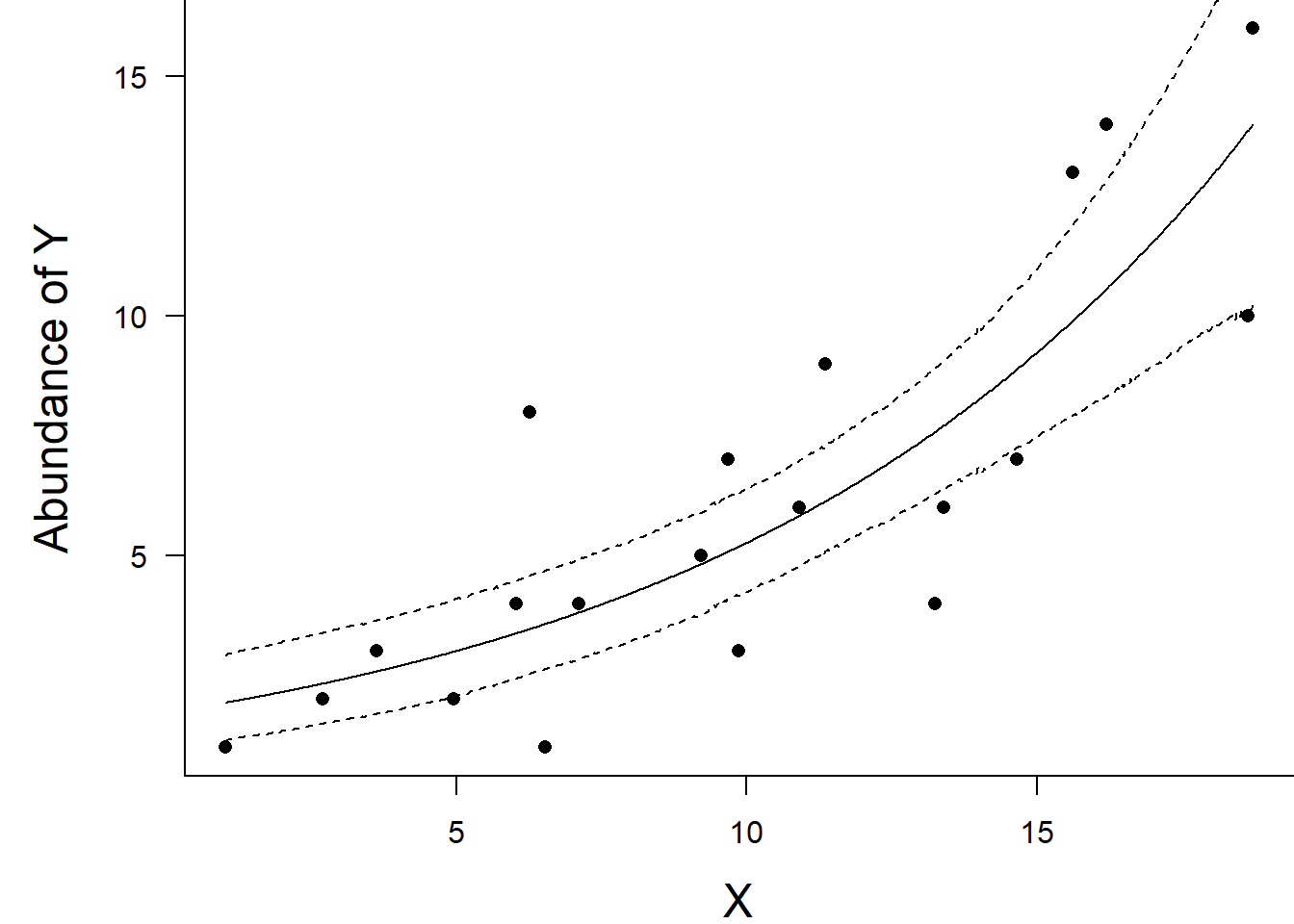
Full log-likelihood function
Now lets try it by specifying log-likelihood and the zero trick. When applying this trick, we need to manually calculate the deviance as the inbuilt deviance will be based on the log-likelihood of estimating the zeros (as part of the zero trick) rather than the deviance of the intended model. The one advantage of the zero trick is that the Deviance and thus DIC, AIC provided by R2jags will be incorrect. Hence, they too need to be manually defined within JAGS I suspect that the AIC calculation I have used is incorrect.
Xmat <- model.matrix(~x, dat)
nX <- ncol(Xmat)
dat.list2 <- with(dat,list(Y=y, X=Xmat,N=nrow(dat), mu=rep(0,nX),
                  Sigma=diag(1.0E-06,nX), zeros=rep(0,nrow(dat)), C=10000))
modelString="
model {
  for (i in 1:N) {
     zeros[i] ~ dpois(zeros.lambda[i])
     zeros.lambda[i] <- -ll[i] + C
     ll[i] <- Y[i]*log(lambda[i]) - lambda[i] - loggam(Y[i]+1)
     eta[i] <- inprod(beta[], X[i,])
     log(lambda[i]) <- eta[i]
    llm[i] <- Y[i]*log(meanlambda) - meanlambda - loggam(Y[i]+1)
  }
  meanlambda <- mean(lambda)
  beta ~ dmnorm(mu[],Sigma[,])
  dev <- sum(-2*ll)
  pD <- mean(dev)-sum(-2*llm)
  AIC <- min(dev+(2*pD))
}
"

writeLines(modelString, con='modelpois_ll.txt')

params <- c('beta','dev','AIC')
nChains = 2
burnInSteps = 5000
thinSteps = 1
numSavedSteps = 20000
nIter = ceiling((numSavedSteps * thinSteps)/nChains)

dat.P.jags3 <- jags(data=dat.list2,model.file='modelpois_ll.txt', param=params,
                   n.chains=nChains, n.iter=nIter, n.burnin=burnInSteps, n.thin=thinSteps)
NA Compiling model graph
NA Resolving undeclared variables
NA Allocating nodes
NA Graph information:
NA Observed stochastic nodes: 20
NA Unobserved stochastic nodes: 1
NA Total graph size: 353
NA
NA Initializing modelprint(dat.P.jags3)NA Inference for Bugs model at "modelpois_ll.txt", fit using jags,
NA 2 chains, each with 10000 iterations (first 5000 discarded)
NA n.sims = 10000 iterations saved
NA mu.vect sd.vect 2.5% 25% 50% 75%
NA AIC 13.728 4.725 9.624 10.548 11.952 15.158
NA beta[1] 0.481 0.259 -0.079 0.319 0.506 0.669
NA beta[2] 0.116 0.019 0.084 0.103 0.114 0.128
NA dev 88.382 2.009 86.361 86.883 87.731 89.265
NA deviance 400088.382 2.009 400086.361 400086.883 400087.731 400089.265
NA 97.5% Rhat n.eff
NA AIC 26.878 1.016 180
NA beta[1] 0.922 1.037 49
NA beta[2] 0.155 1.029 60
NA dev 94.071 1.009 300
NA deviance 400094.071 1.000 1
NA
NA For each parameter, n.eff is a crude measure of effective sample size,
NA and Rhat is the potential scale reduction factor (at convergence, Rhat=1).
NA
NA DIC info (using the rule, pD = var(deviance)/2)
NA pD = 2.0 and DIC = 400090.4
NA DIC is an estimate of expected predictive error (lower deviance is better).Negative binomial
The following equations are provided since in Bayesian modelling, it is occasionally necessary to directly define the log-likelihood calculations (particularly for zero-inflated models and other mixture models).
\[ f(y \mid r, p) = \frac{\Gamma(y+r)}{\Gamma(r)\Gamma(y+1)}p^r(1-p)^y, \]
where \(p\) is the probability of \(y\) successes until \(r\) failures. If, we make \(p=\frac{\text{size}}{\text{size}+\mu}\), then we can define the function in terms of \(\mu\):
\[ \mu = \frac{r(1-p)}{p}, \]
where \(E[Y]=\mu\), \(Var(Y)=\mu + \frac{\mu^2}{r}\).
Data generation
Lets say we wanted to model the abundance of an item (\(y\)) against a continuous predictor (\(x\)). As this section is mainly about the generation of artificial data (and not specifically about what to do with the data), understanding the actual details are optional and can be safely skipped.
set.seed(37) #16 #35
#The number of samples
n.x <- 20
#Create x values that at uniformly distributed throughout the rate of 1 to 20
x <- sort(runif(n = n.x, min = 1, max =20))
mm <- model.matrix(~x)
intercept <- 0.6
slope=0.1
#The linear predictor
linpred <- mm %*% c(intercept,slope)
#Predicted y values
lambda <- exp(linpred)
#Add some noise and make binomial
y <- rnbinom(n=n.x, mu=lambda, size=1)
dat.nb <- data.frame(y,x)
When counts are all very large (not close to \(0\)) and their ranges do not span orders of magnitude, they take on very Gaussian properties (symmetrical distribution and variance independent of the mean). Given that models based on the Gaussian distribution are more optimized and recognized than Generalized Linear Models, it can be prudent to adopt Gaussian models for such data. Hence it is a good idea to first explore whether a Poisson or Negative Binomial model is likely to be more appropriate than a standard Gaussian model. Recall from Poisson regression, there are five main potential models that we could consider fitting to these data.
hist(dat$x)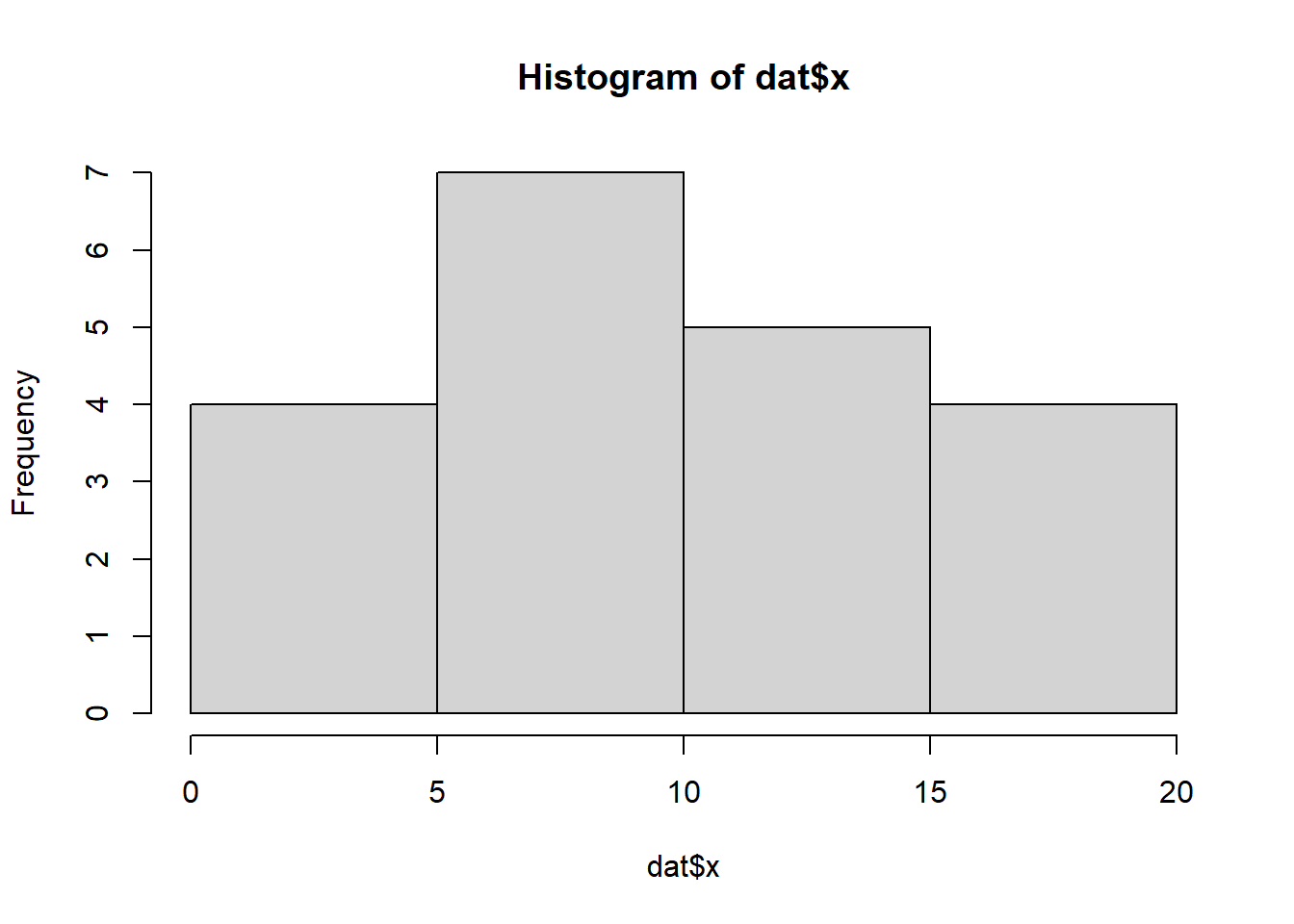
#now for the scatterplot
plot(y~x, dat.nb, log="y")
with(dat.nb, lines(lowess(y~x)))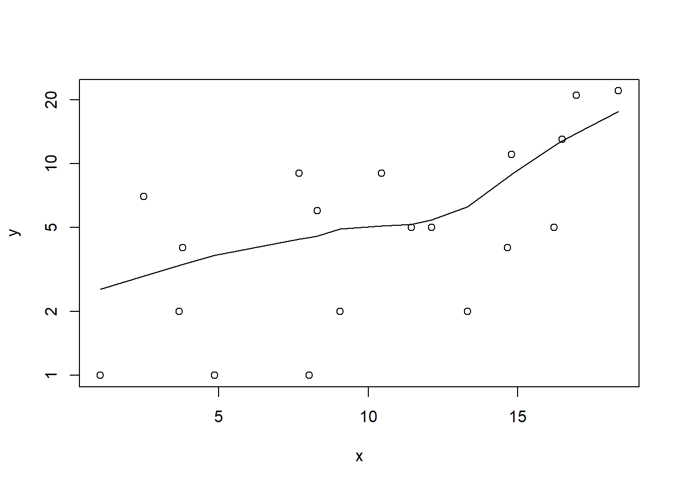
Conclusions: the predictor (\(x\)) does not display any skewness or other issues that might lead to non-linearity. The lowess smoother on the scatterplot does not display major deviations from a straight line and thus linearity is satisfied. Violations of linearity could be addressed by either:
define a non-linear linear predictor (such as a polynomial, spline or other non-linear function).
transform the scale of the predictor variables.
Although we have already established that there are few zeros in the data (and thus overdispersion is unlikely to be an issue), we can also explore this by comparing the number of zeros in the data to the number of zeros that would be expected from a Poisson distribution with a mean equal to the mean count of the data.
#proportion of 0's in the data
dat.nb.tab<-table(dat.nb$y==0)
dat.nb.tab/sum(dat.nb.tab)
NA
NA FALSE TRUE
NA 0.95 0.05#proportion of 0's expected from a Poisson distribution
mu <- mean(dat.nb$y)
cnts <- rpois(1000, mu)
dat.nb.tabE <- table(cnts == 0)
dat.nb.tabE/sum(dat.nb.tabE)NA
NA FALSE
NA 1In the above, the value under FALSE is the proportion of non-zero values in the data and the value under TRUE is the proportion of zeros in the data. In this example, the proportion of zeros observed is similar to the proportion expected. Indeed, there was only a single zero observed. Hence it is likely that if there is overdispersion it is unlikely to be due to excessive zeros.
Model fitting
\[ y_i \sim \text{NegBin}(p_i,r), \]
where \(p_i=\frac{r}{r+\lambda_i}\), with \(\log(\lambda_i)=\beta_0+\beta_1x_{i}\) and \(\beta_0,\beta_1 \sim N(0, 10000)\), \(r \sim \text{Unif}(0.001,1000)\).
dat.nb.list <- with(dat.nb,list(Y=y, X=x,N=nrow(dat.nb)))
modelString="
model {
  for (i in 1:N) {
     Y[i] ~ dnegbin(p[i],size)
     p[i] <- size/(size+lambda[i])
     log(lambda[i]) <- beta0 + beta1*X[i]
  }
  beta0 ~ dnorm(0,1.0E-06)
  beta1 ~ dnorm(0,1.0E-06)
  size ~ dunif(0.001,1000)
  theta <- pow(1/mean(p),2)
  scaleparam <- mean((1-p)/p)
}
"
writeLines(modelString, con='modelnbin.txt')

params <- c('beta0','beta1', 'size','theta','scaleparam')
nChains = 2
burnInSteps = 5000
thinSteps = 1
numSavedSteps = 20000
nIter = ceiling((numSavedSteps * thinSteps)/nChains)

dat.NB.jags <- jags(data=dat.nb.list,model.file='modelnbin.txt', param=params,
                   n.chains=nChains, n.iter=nIter, n.burnin=burnInSteps, n.thin=thinSteps)
NA Compiling model graph
NA Resolving undeclared variables
NA Allocating nodes
NA Graph information:
NA Observed stochastic nodes: 20
NA Unobserved stochastic nodes: 3
NA Total graph size: 157
NA
NA Initializing modelModel evaluation
denplot(dat.NB.jags, parms = c("beta0","beta1","size"))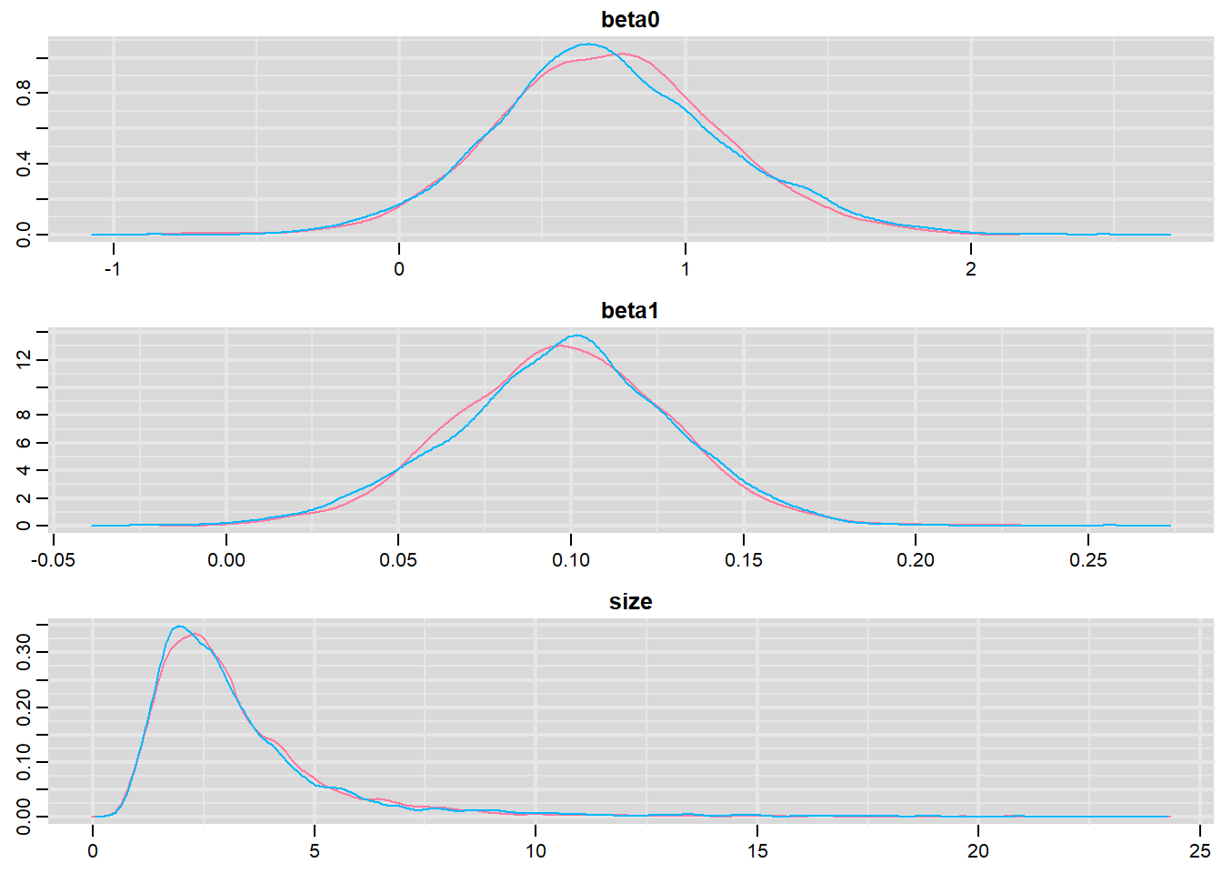
traplot(dat.NB.jags, parms = c("beta0","beta1","size"))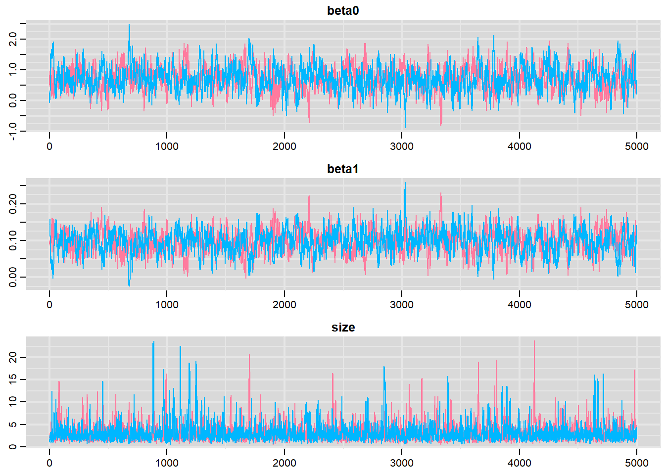
raftery.diag(as.mcmc(dat.NB.jags))NA [[1]]
NA
NA Quantile (q) = 0.025
NA Accuracy (r) = +/- 0.005
NA Probability (s) = 0.95
NA
NA Burn-in Total Lower bound Dependence
NA (M) (N) (Nmin) factor (I)
NA beta0 16 17518 3746 4.68
NA beta1 24 28713 3746 7.66
NA deviance 3 4198 3746 1.12
NA scaleparam 16 16290 3746 4.35
NA size 4 5038 3746 1.34
NA theta 16 16244 3746 4.34
NA
NA
NA [[2]]
NA
NA Quantile (q) = 0.025
NA Accuracy (r) = +/- 0.005
NA Probability (s) = 0.95
NA
NA Burn-in Total Lower bound Dependence
NA (M) (N) (Nmin) factor (I)
NA beta0 18 20025 3746 5.35
NA beta1 24 21072 3746 5.63
NA deviance 3 4267 3746 1.14
NA scaleparam 18 19920 3746 5.32
NA size 3 4375 3746 1.17
NA theta 20 20682 3746 5.52autocorr.diag(as.mcmc(dat.NB.jags))NA beta0 beta1 deviance scaleparam size
NA Lag 0 1.000000000 1.000000000 1.000000000 1.00000000 1.000000000
NA Lag 1 0.855250119 0.856542892 0.566377262 0.33360033 0.684520361
NA Lag 5 0.519024321 0.521535488 0.163024546 0.07618281 0.220180993
NA Lag 10 0.276801196 0.280283232 0.025179110 0.02814049 0.039259726
NA Lag 50 -0.008060569 -0.004454124 -0.003876422 -0.01103395 0.006904325
NA theta
NA Lag 0 1.00000000
NA Lag 1 0.26024619
NA Lag 5 0.05872969
NA Lag 10 0.02940084
NA Lag 50 -0.01349378We now explore the goodness of fit of the models via the residuals and deviance. We could calculate the Pearsons’s residuals within the JAGS model. Alternatively, we could use the parameters to generate the residuals outside of JAGS.
#extract the samples for the two model parameters
coefs <- dat.NB.jags$BUGSoutput$sims.matrix[,1:2]
size <- dat.NB.jags$BUGSoutput$sims.matrix[,'size']
Xmat <- model.matrix(~x, data=dat.nb)
#expected values on a log scale
eta<-coefs %*% t(Xmat)
#expected value on response scale
lambda <- exp(eta)
varY <- lambda + (lambda^2)/size
#sweep across rows and then divide by lambda
Resid <- -1*sweep(lambda,2,dat.nb$y,'-')/sqrt(varY)
#plot residuals vs expected values
plot(apply(Resid,2,mean)~apply(eta,2,mean))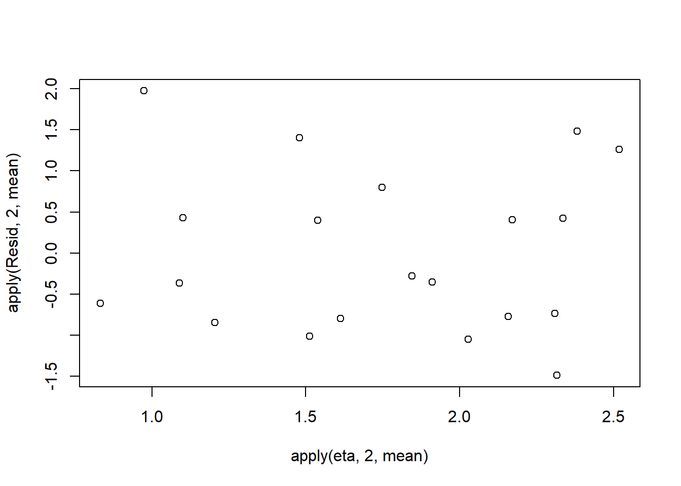
Now we will compare the sum of squared residuals to the sum of squares residuals that would be expected from a Negative binomial distribution matching that estimated by the model. Essentially this is estimating how well the Negative binomial distribution, the log-link function and the linear model approximates the observed data.
SSres<-apply(Resid^2,1,sum)

#generate a matrix of draws from a negative binomial distribution
# the matrix is the same dimensions as pi and uses the probabilities of pi
YNew <- matrix(rnbinom(length(lambda),mu=lambda, size=size),nrow=nrow(lambda))
Resid1<-(lambda - YNew)/sqrt(varY)
SSres.sim<-apply(Resid1^2,1,sum)
mean(SSres.sim>SSres, na.rm = T)
NA [1] 0.4163Conclusions: the Bayesian p-value is approximately \(0.5\), suggesting that there is a good fit of the model to the data.
Unfortunately, unlike with linear models (Gaussian family), the expected distribution of data (residuals) varies over the range of fitted values for numerous (often competing) ways that make diagnosing (and attributing causes thereof) miss-specified generalized linear models from standard residual plots very difficult. The use of standardized (Pearson) residuals or deviance residuals can partly address this issue, yet they still do not offer completely consistent diagnoses across all issues (miss-specified model, over-dispersion, zero-inflation). An alternative approach is to use simulated data from the model posteriors to calculate an empirical cumulative density function from which residuals are are generated as values corresponding to the observed data along the density function.
#extract the samples for the two model parameters
coefs <- dat.NB.jags$BUGSoutput$sims.matrix[,1:2]
size <- dat.NB.jags$BUGSoutput$sims.matrix[,'size']
Xmat <- model.matrix(~x, data=dat.nb)
#expected values on a log scale
eta<-coefs %*% t(Xmat)
#expected value on response scale
lambda <- exp(eta)

simRes <- function(lambda, data,n=250, plot=T, family='negbin', size=NULL) {
 require(gap)
 N = nrow(data)
 sim = switch(family,
    'poisson' = matrix(rpois(n*N,apply(lambda,2,mean)),ncol=N, byrow=TRUE),
    'negbin' = matrix(MASS:::rnegbin(n*N,apply(lambda,2,mean),size),ncol=N, byrow=TRUE)
 )
 a = apply(sim + runif(n,-0.5,0.5),2,ecdf)
 resid<-NULL
 for (i in 1:nrow(data)) resid<-c(resid,a[[i]](data$y[i] + runif(1 ,-0.5,0.5)))
 if (plot==T) {
   par(mfrow=c(1,2))
   gap::qqunif(resid,pch = 2, bty = "n",
   logscale = F, col = "black", cex = 0.6, main = "QQ plot residuals",
   cex.main = 1, las=1)
   plot(resid~apply(lambda,2,mean), xlab='Predicted value', ylab='Standardized residual', las=1)
 }
 resid
}

simRes(lambda,dat.nb, family='negbin', size=mean(size))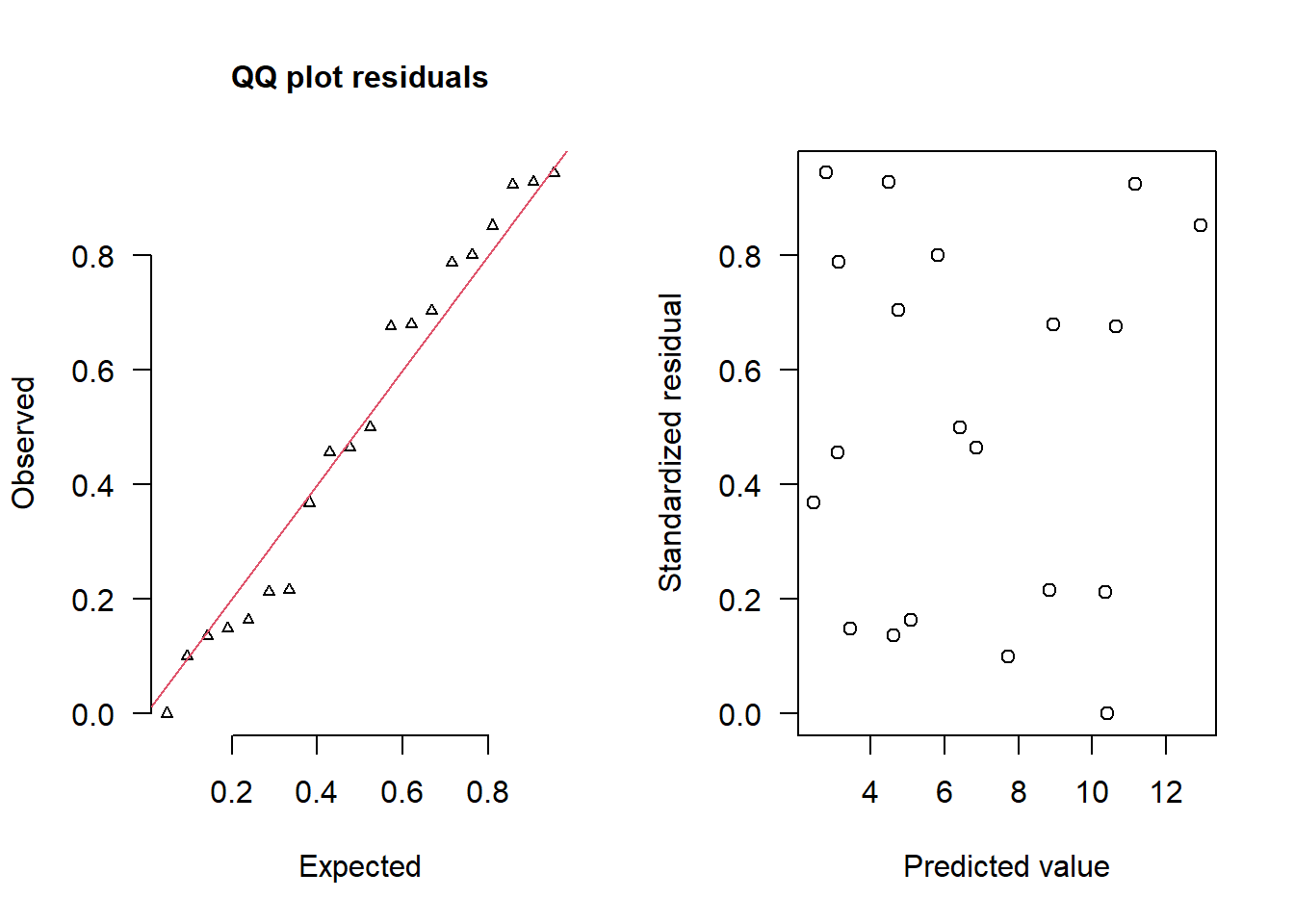
NA  [1] 0.368 0.944 0.456 0.788 0.148 0.928 0.136 0.704 0.164 0.800 0.500 0.464
NA [13] 0.100 0.216 0.680 0.212 0.000 0.676 0.924 0.852
The trend (black symbols) in the qq-plot does not appear to be overly non-linear (matching the ideal red line well), suggesting that the model is not overdispersed. The spread of standardized (simulated) residuals in the residual plot do not appear overly non-uniform. That is there is not trend in the residuals. Furthermore, there is not a concentration of points close to \(1\) or \(0\) (which would imply overdispersion).
Exploring the model parameters
If there was any evidence that the assumptions had been violated or the model was not an appropriate fit, then we would need to reconsider the model and start the process again. In this case, there is no evidence that the test will be unreliable so we can proceed to explore the test statistics. As with most Bayesian models, it is best to base conclusions on medians rather than means.
print(dat.NB.jags)NA Inference for Bugs model at "modelnbin.txt", fit using jags,
NA 2 chains, each with 10000 iterations (first 5000 discarded)
NA n.sims = 10000 iterations saved
NA mu.vect sd.vect 2.5% 25% 50% 75% 97.5% Rhat n.eff
NA beta0 0.731 0.395 -0.023 0.470 0.717 0.984 1.534 1.001 10000
NA beta1 0.097 0.032 0.034 0.077 0.098 0.118 0.158 1.001 10000
NA scaleparam 2.787 1.756 0.704 1.670 2.412 3.444 7.089 1.001 10000
NA size 3.255 2.190 1.055 1.941 2.697 3.853 9.050 1.001 10000
NA theta 12.548 12.474 2.669 5.892 9.157 14.790 43.249 1.001 10000
NA deviance 113.053 2.691 110.093 111.115 112.352 114.190 120.305 1.002 2000
NA
NA For each parameter, n.eff is a crude measure of effective sample size,
NA and Rhat is the potential scale reduction factor (at convergence, Rhat=1).
NA
NA DIC info (using the rule, pD = var(deviance)/2)
NA pD = 3.6 and DIC = 116.7
NA DIC is an estimate of expected predictive error (lower deviance is better).adply(dat.NB.jags$BUGSoutput$sims.matrix, 2, function(x) {
data.frame(Median=median(x), Mean=mean(x), HPDinterval(as.mcmc(x)), HPDinterval(as.mcmc(x),p=0.5))
})NA X1 Median Mean lower upper lower.1
NA 1 beta0 0.71693048 0.73121205 -0.05129743 1.5032427 0.4523583
NA 2 beta1 0.09800852 0.09730699 0.03509028 0.1591976 0.0789372
NA 3 deviance 112.35178835 113.05255254 109.86520971 118.4814291 110.0898498
NA 4 scaleparam 2.41198253 2.78665197 0.33094006 5.9583607 1.2865037
NA 5 size 2.69653197 3.25545915 0.68960555 7.2146030 1.4202953
NA 6 theta 9.15704708 12.54776430 1.61632232 32.9116959 3.6489231
NA upper.1
NA 1 0.9610028
NA 2 0.1201659
NA 3 112.4668566
NA 4 2.8677393
NA 5 2.9988148
NA 6 10.3646959#on original scale
adply(exp(dat.NB.jags$BUGSoutput$sims.matrix[,1:2]), 2, function(x) {
data.frame(Median=median(x), Mean=mean(x), HPDinterval(as.mcmc(x)), HPDinterval(as.mcmc(x),p=0.5))
})NA X1 Median Mean lower upper lower.1 upper.1
NA 1 beta0 2.048137 2.249960 0.8335273 4.249614 1.340384 2.309801
NA 2 beta1 1.102972 1.102753 1.0357132 1.172570 1.080463 1.125944Conclusions: We would reject the null hypothesis of no effect of \(x\) on \(y\). An increase in x is associated with a significant linear increase (positive slope) in the abundance of \(y\). Every \(1\) unit increase in \(x\) results in a log \(0.09\) unit increase in \(y\). We usually express this in terms of abundance rather than log abundance, so every \(1\) unit increase in \(x\) results in a ($e^{ 0.09} = 1.02 $) \(1.02\) unit increase in the abundance of \(y\).
Explorations of the trends
A measure of the strength of the relationship can be obtained according to:
\[ R^2 = 1 - \frac{\text{RSS}_{model}}{\text{RSS}_{null}} \]
Xmat <- model.matrix(~x, data=dat.nb)
#expected values on a log scale
eta<-coefs %*% t(Xmat)
#expected value on response scale
lambda <- exp(eta)
#calculate the raw SS residuals
SSres <- apply((-1*(sweep(lambda,2,dat.nb$y,'-')))^2,1,sum)
SSres.null <- sum((dat.nb$y - mean(dat.nb$y))^2)
#OR
SSres.null <- crossprod(dat.nb$y - mean(dat.nb$y))
#calculate the model r2
1-mean(SSres)/SSres.null
NA [,1]
NA [1,] 0.270553Conclusions: \(27\)% of the variation in \(y\) abundance can be explained by its relationship with \(x\). We can also do it directly into JAGS.
Finally, we will create a summary plot.
par(mar = c(4, 5, 0, 0))
plot(y ~ x, data = dat.nb, type = "n", ann = F, axes = F)
points(y ~ x, data = dat.nb, pch = 16)
xs <- seq(min(dat.nb$x,na.rm=TRUE),max(dat.nb$x,na.rm=TRUE), l = 1000)
Xmat <- model.matrix(~xs)
eta<-coefs %*% t(Xmat)
ys <- exp(eta)
library(plyr)
library(coda)
data.tab <- adply(ys,2,function(x) {
  data.frame(Median=median(x), HPDinterval(as.mcmc(x)))
})
data.tab <- cbind(x=xs,data.tab)
points(Median ~ x, data=data.tab,col = "black", type = "l")
lines(lower ~ x, data=data.tab,col = "black", type = "l", lty = 2)
lines(upper ~ x, data=data.tab,col = "black", type = "l", lty = 2)

axis(1)
mtext("X", 1, cex = 1.5, line = 3)
axis(2, las = 2)
mtext("Abundance of Y", 2, cex = 1.5, line = 3)
box(bty = "l")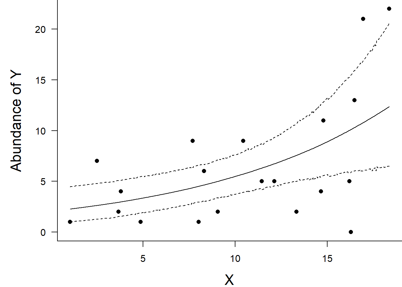
Full log-likelihood function
Now lets try it by specifying log-likelihood and the zero trick. When applying this trick, we need to manually calculate the deviance as the inbuilt deviance will be based on the log-likelihood of estimating the zeros (as part of the zero trick) rather than the deviance of the intended model. The one advantage of the zero trick is that the Deviance and thus DIC, AIC provided by R2jags will be incorrect. Hence, they too need to be manually defined within JAGS I suspect that the AIC calculation I have used is incorrect.
Xmat <- model.matrix(~x, dat.nb)
nX <- ncol(Xmat)
dat.nb.list2 <- with(dat.nb,list(Y=y, X=Xmat,N=nrow(dat.nb), mu=rep(0,nX),
                  Sigma=diag(1.0E-06,nX), zeros=rep(0,nrow(dat.nb)), C=10000))
modelString="
model {
  for (i in 1:N) {
     zeros[i] ~ dpois(zeros.lambda[i])
     zeros.lambda[i] <- -ll[i] + C
     ll[i] <- loggam(Y[i]+size) - loggam(Y[i]+1) - loggam(size) + size*(log(p[i]) - log(p[i]+1)) -
              Y[i]*log(p[i]+1)
     p[i] <- size/lambda[i]
     eta[i] <- inprod(beta[], X[i,])
     log(lambda[i]) <- eta[i]
  }
  beta ~ dmnorm(mu[],Sigma[,])
  size ~ dunif(0.001,1000)
  dev <- sum(-2*ll)
}
"

writeLines(modelString, con='modelnbin_ll.txt')

params <- c('beta','dev')
nChains = 2
burnInSteps = 5000
thinSteps = 1
numSavedSteps = 20000
nIter = ceiling((numSavedSteps * thinSteps)/nChains)

dat.NB.jags3 <- jags(data=dat.nb.list2,model.file='modelnbin_ll.txt', param=params,
                   n.chains=nChains, n.iter=nIter, n.burnin=burnInSteps, n.thin=thinSteps)
NA Compiling model graph
NA Resolving undeclared variables
NA Allocating nodes
NA Graph information:
NA Observed stochastic nodes: 20
NA Unobserved stochastic nodes: 2
NA Total graph size: 453
NA
NA Initializing modelprint(dat.NB.jags3)NA Inference for Bugs model at "modelnbin_ll.txt", fit using jags,
NA 2 chains, each with 10000 iterations (first 5000 discarded)
NA n.sims = 10000 iterations saved
NA mu.vect sd.vect 2.5% 25% 50% 75%
NA beta[1] 0.739 0.386 0.039 0.484 0.726 0.968
NA beta[2] 0.096 0.031 0.034 0.077 0.096 0.116
NA dev 112.830 2.548 110.074 111.037 112.105 113.842
NA deviance 400112.830 2.548 400110.074 400111.037 400112.105 400113.842
NA 97.5% Rhat n.eff
NA beta[1] 1.536 1.015 160
NA beta[2] 0.153 1.010 230
NA dev 119.701 1.002 1200
NA deviance 400119.701 1.000 1
NA
NA For each parameter, n.eff is a crude measure of effective sample size,
NA and Rhat is the potential scale reduction factor (at convergence, Rhat=1).
NA
NA DIC info (using the rule, pD = var(deviance)/2)
NA pD = 3.2 and DIC = 400116.1
NA DIC is an estimate of expected predictive error (lower deviance is better).Zero inflated Poisson
Zero-Inflation Poisson (ZIP) mixture model is defined as:
\[ p(y_i \mid \theta, \lambda) = \begin{cases} \theta + (1-\theta) \times \text{Pois}(0 \mid \lambda) & \text{if } y_i = 0\\ (1-\theta) \times \text{Pois}(y_i \mid \lambda) & \text{if } y_i > 0, \end{cases} \]
where \(\theta\) is the probability of false values (zeros). Hence there is essentially two models coupled together (a mixture model) to yield an overall probability:
when an observed response is zero (\(y_i=0\)), it is the probability of getting a false value (zero) plus the probability of a true value multiplied probability of drawing a value of zero from a Poisson distribution of lambda.
when an observed response is greater than \(0\), it is the probability of a true value multiplied probability of drawing that value from a Poisson distribution of lambda
The above formulation indicates the same \(\lambda\) for both the zeros and non-zeros components. In the model of zero values, we are essentially investigating whether the likelihood of false zeros is related to the linear predictor and then the greater than zero model investigates whether the counts are related to the linear predictor. However, we are typically less interested in modelling determinants of false zeros. Indeed, it is better that the likelihood of false zeros be unrelated to the linear predictor. For example, if excess (false zeros) are due to issues of detectability (individuals are present, just not detected), it is better that the detectability is not related to experimental treatments. Ideally, any detectability issues should be equal across all treatment levels. The expected value of \(Y\) and the variance in \(Y\) for a ZIP model are:
\[ E[y_i] = \lambda \times (1-\theta), \]
\[ \text{Var}(y_i) = \lambda \times (1-\theta) \times (1+\theta \times \lambda^2) \]
Data generation
Lets say we wanted to model the abundance of an item (\(y\)) against a continuous predictor (\(x\)). As this section is mainly about the generation of artificial data (and not specifically about what to do with the data), understanding the actual details are optional and can be safely skipped.
set.seed(9) #34.5  #4 #10 #16 #17 #26
#The number of samples
n.x <- 20
#Create x values that at uniformly distributed throughout the rate of 1 to 20
x <- sort(runif(n = n.x, min = 1, max =20))
mm <- model.matrix(~x)
intercept <- 0.6
slope=0.1
#The linear predictor
linpred <- mm %*% c(intercept,slope)
#Predicted y values
lambda <- exp(linpred)
#Add some noise and make binomial
library(gamlss.dist)
#fixed latent binomial
y<- rZIP(n.x,lambda, 0.4)
#latent binomial influenced by the linear predictor
#y<- rZIP(n.x,lambda, 1-exp(linpred)/(1+exp(linpred)))
dat.zip <- data.frame(y,x)

summary(glm(y~x, dat.zip, family="poisson"))
NA
NA Call:
NA glm(formula = y ~ x, family = "poisson", data = dat.zip)
NA
NA Coefficients:
NA Estimate Std. Error z value Pr(>|z|)
NA (Intercept) 0.30200 0.25247 1.196 0.232
NA x 0.10691 0.01847 5.789 7.09e-09 ***
NA ---
NA Signif. codes: 0 '***' 0.001 '**' 0.01 '*' 0.05 '.' 0.1 ' ' 1
NA
NA (Dispersion parameter for poisson family taken to be 1)
NA
NA Null deviance: 111.495 on 19 degrees of freedom
NA Residual deviance: 79.118 on 18 degrees of freedom
NA AIC: 126.64
NA
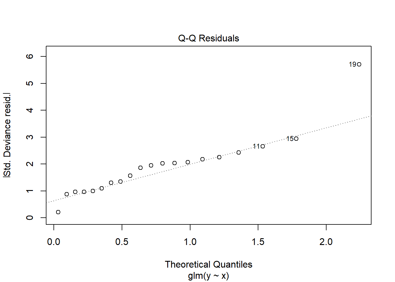
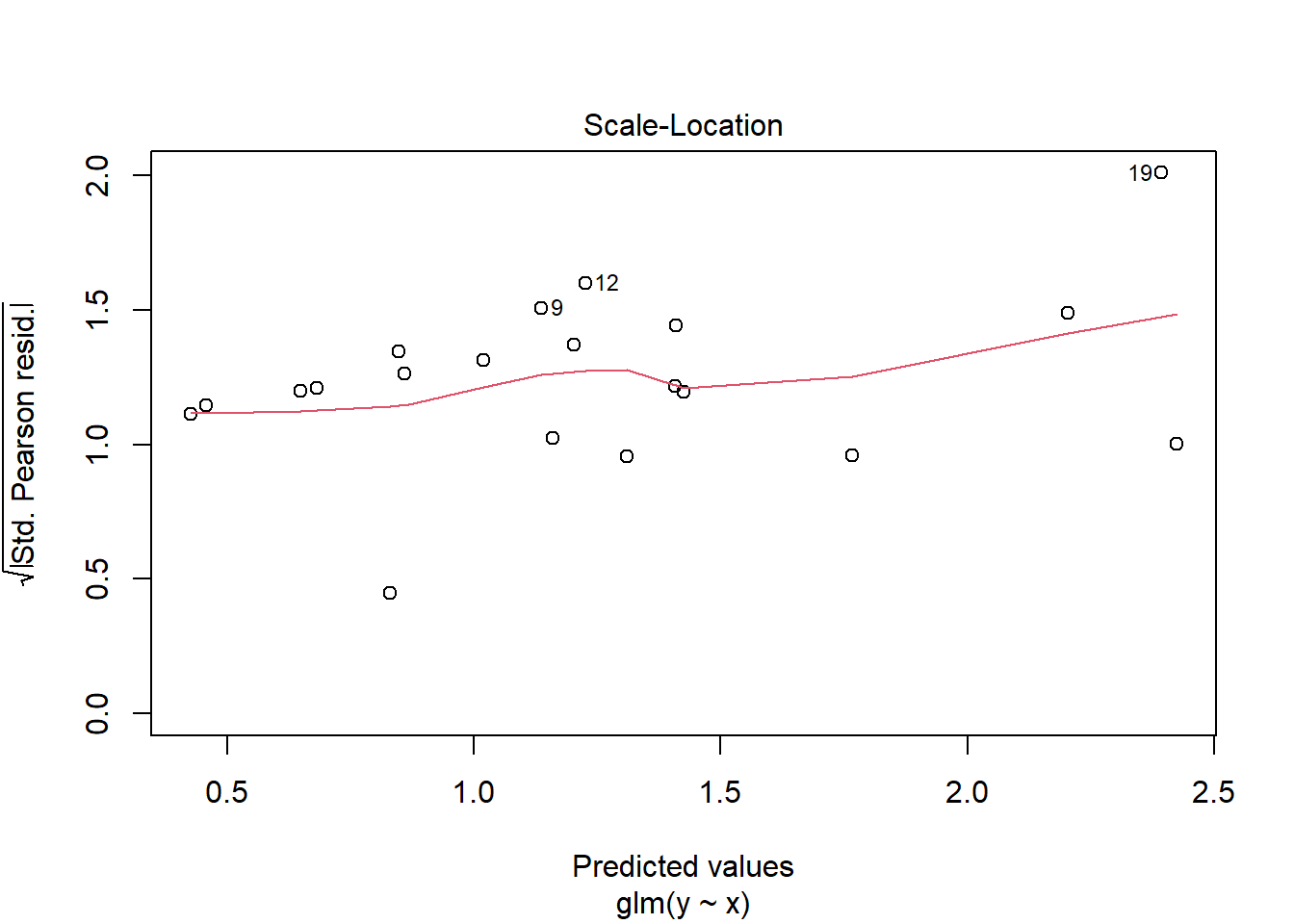
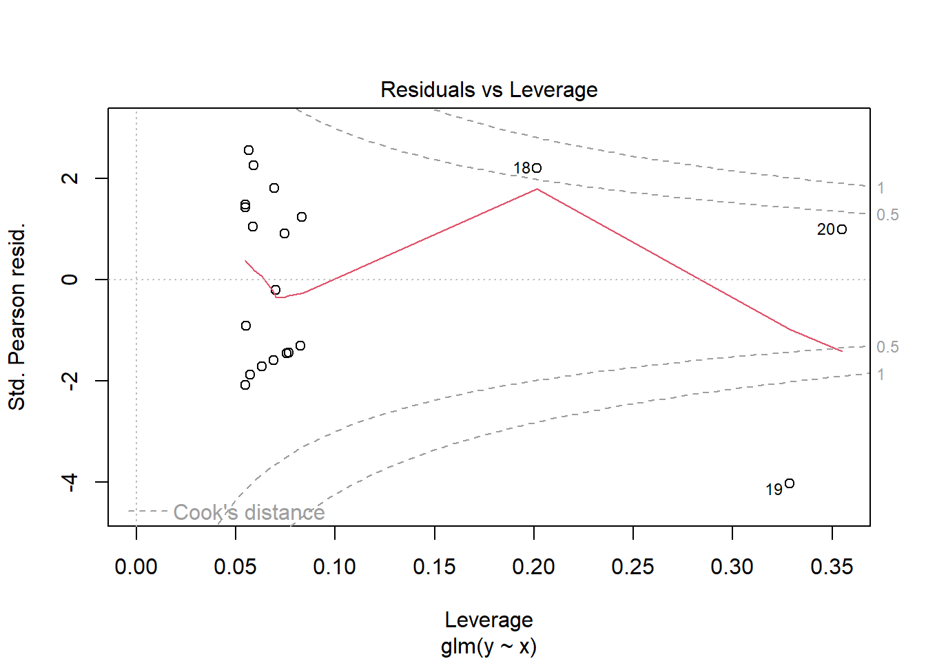
NA Number of Fisher Scoring iterations: 5plot(glm(y~x, dat.zip, family="poisson"))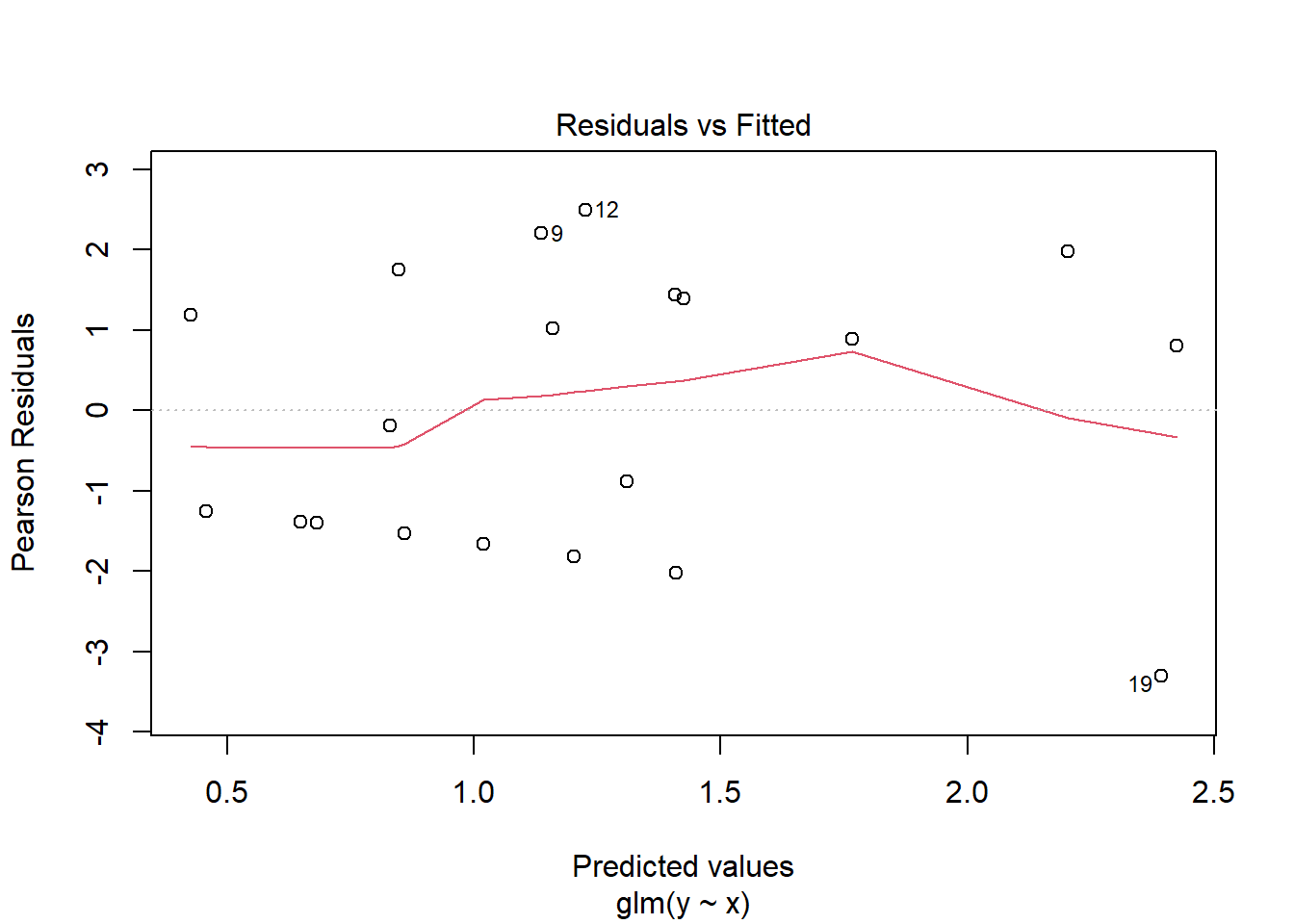
library(pscl)
summary(zeroinfl(y ~ x | 1, dist = "poisson", data = dat.zip))
NA
NA Call:
NA zeroinfl(formula = y ~ x | 1, data = dat.zip, dist = "poisson")
NA
NA Pearson residuals:
NA Min 1Q Median 3Q Max
NA -1.1625 -0.9549 0.1955 0.8125 1.4438
NA
NA Count model coefficients (poisson with log link):
NA Estimate Std. Error z value Pr(>|z|)
NA (Intercept) 0.88696 0.28825 3.077 0.00209 **
NA x 0.09374 0.02106 4.450 8.58e-06 ***
NA
NA Zero-inflation model coefficients (binomial with logit link):
NA Estimate Std. Error z value Pr(>|z|)
NA (Intercept) -0.4581 0.4725 -0.97 0.332
NA ---
NA Signif. codes: 0 '***' 0.001 '**' 0.01 '*' 0.05 '.' 0.1 ' ' 1
NA
NA Number of iterations in BFGS optimization: 8
NA Log-likelihood: -38.58 on 3 Dfplot(resid(zeroinfl(y ~ x | 1, dist = "poisson", data = dat.zip))~fitted(zeroinfl(y ~ x | 1, dist = "poisson")))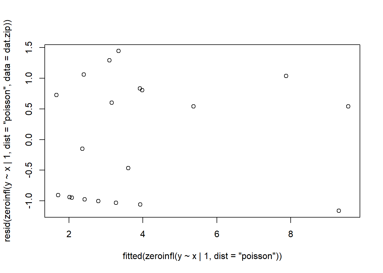
library(gamlss)
summary(gamlss(y~x,data=dat.zip, family=ZIP))
NA GAMLSS-RS iteration 1: Global Deviance = 77.8434
NA GAMLSS-RS iteration 2: Global Deviance = 77.1603
NA GAMLSS-RS iteration 3: Global Deviance = 77.1598
NA ******************************************************************
NA Family: c("ZIP", "Poisson Zero Inflated")
NA
NA Call: gamlss(formula = y ~ x, family = ZIP, data = dat.zip)
NA
NA Fitting method: RS()
NA
NA ------------------------------------------------------------------
NA Mu link function: log
NA Mu Coefficients:
NA Estimate Std. Error t value Pr(>|t|)
NA (Intercept) 0.88620 0.28819 3.075 0.006862 **
NA x 0.09387 0.02105 4.458 0.000345 ***
NA ---
NA Signif. codes: 0 '***' 0.001 '**' 0.01 '*' 0.05 '.' 0.1 ' ' 1
NA
NA ------------------------------------------------------------------
NA Sigma link function: logit
NA Sigma Coefficients:
NA Estimate Std. Error t value Pr(>|t|)
NA (Intercept) -0.4582 0.4725 -0.97 0.346
NA
NA ------------------------------------------------------------------
NA No. of observations in the fit: 20
NA Degrees of Freedom for the fit: 3
NA Residual Deg. of Freedom: 17
NA at cycle: 3
NA
NA Global Deviance: 77.15981
NA AIC: 83.15981
NA SBC: 86.14701
NA ******************************************************************predict(gamlss(y~x,data=dat.zip, family=ZIP), se.fit=TRUE, what="mu")NA GAMLSS-RS iteration 1: Global Deviance = 77.8434
NA GAMLSS-RS iteration 2: Global Deviance = 77.1603
NA GAMLSS-RS iteration 3: Global Deviance = 77.1598NA $fit
NA 1 2 3 4 5 6 7 8
NA 0.9952647 1.0233409 1.1897115 1.2189891 1.3490911 1.3644351 1.3748867 1.5164069
NA 9 10 11 12 13 14 15 16
NA 1.6184170 1.6379917 1.6760055 1.6962694 1.7705249 1.8559090 1.8578379 1.8718850
NA 17 18 19 20
NA 2.1712345 2.5536059 2.7205304 2.7472964
NA
NA $se.fit
NA 1 2 3 4 5 6 7 8
NA 0.3826655 0.3724115 0.3131865 0.3031078 0.2601025 0.2552658 0.2520053 0.2112310
NA 9 10 11 12 13 14 15 16
NA 0.1872286 0.1833232 0.1765049 0.1733169 0.1646100 0.1610460 0.1610499 0.1611915
NA 17 18 19 20
NA 0.2055555 0.3248709 0.3848647 0.3947072Exploratory data analysis
Check the distribution of the \(y\) abundances.
hist(dat.zip$y)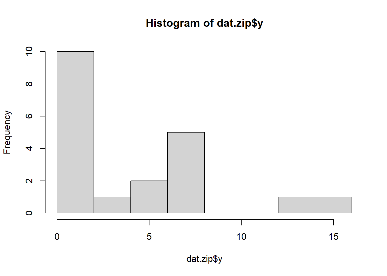
boxplot(dat.zip$y, horizontal=TRUE)
rug(jitter(dat.zip$y))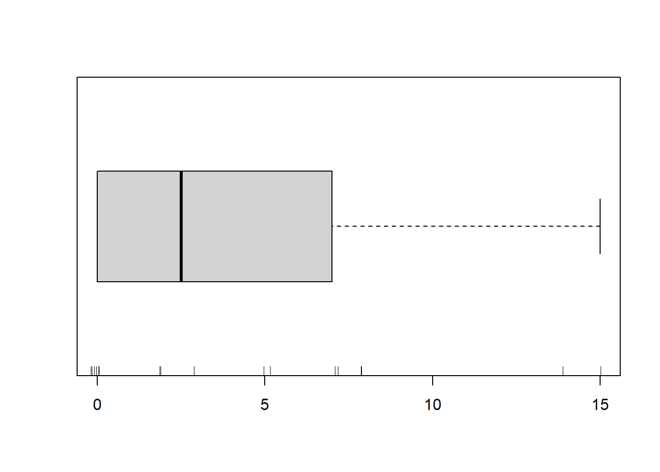
There is definitely signs of non-normality that would warrant Poisson models. Further to that, there appears to be a large number of zeros that are likely to be the cause of overdispersion A zero-inflated Poisson model is likely to be one of the most effective for modeling these data. Lets now explore linearity by creating a histogram of the predictor variable (\(x\)). Note, it is difficult to directly assess issues of linearity. Indeed, a scatterplot with lowess smoother will be largely influenced by the presence of zeros. One possible way of doing so is to explore the trend in the non-zero data.
hist(dat.zip$x)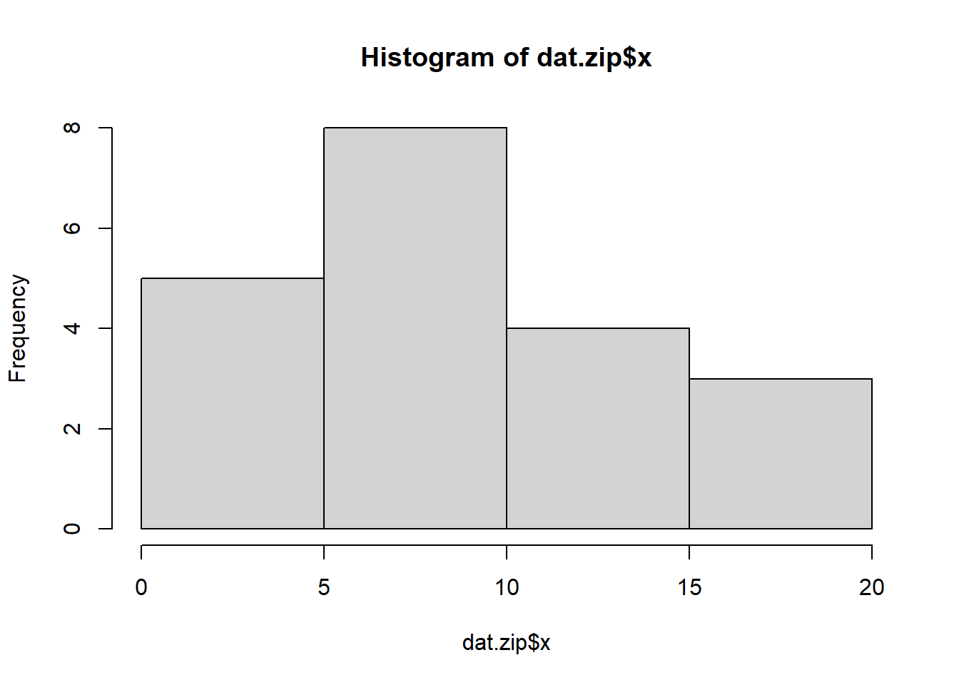
#now for the scatterplot
plot(y~x, dat.zip)
with(subset(dat.zip,y>0), lines(lowess(y~x)))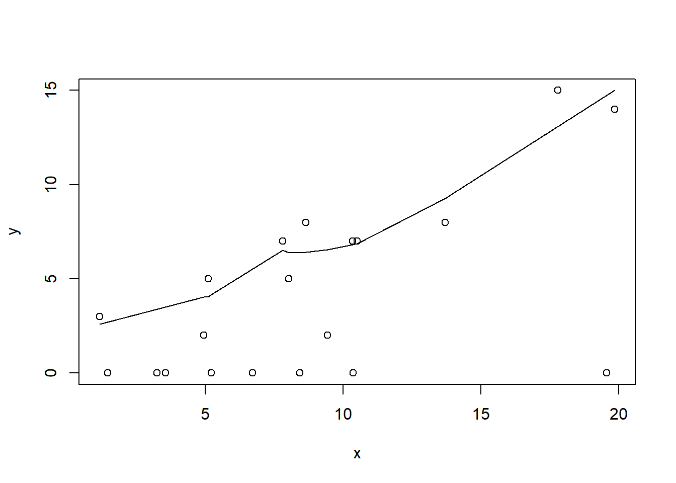
Conclusions: the predictor (\(x\)) does not display any skewness or other issues that might lead to non-linearity. The lowess smoother on the non-zero data cloud does not display major deviations from a straight line and thus linearity is likely to be satisfied. Violations of linearity (whilst difficult to be certain about due to the unknown influence of the zeros) could be addressed by either:
define a non-linear linear predictor (such as a polynomial, spline or other non-linear function).
transform the scale of the predictor variables.
Although we have already established that there are few zeros in the data (and thus overdispersion is unlikely to be an issue), we can also explore this by comparing the number of zeros in the data to the number of zeros that would be expected from a Poisson distribution with a mean equal to the mean count of the data.
#proportion of 0's in the data
dat.zip.tab<-table(dat.zip$y==0)
dat.zip.tab/sum(dat.zip.tab)
NA
NA FALSE TRUE
NA 0.6 0.4#proportion of 0's expected from a Poisson distribution
mu <- mean(dat.zip$y)
cnts <- rpois(1000, mu)
dat.zip.tabE <- table(cnts == 0)
dat.zip.tabE/sum(dat.zip.tabE)NA
NA FALSE TRUE
NA 0.982 0.018In the above, the value under FALSE is the proportion of non-zero values in the data and the value under TRUE is the proportion of zeros in the data. In this example, the proportion of zeros observed (\(45\)%) far exceeds that that would have been expected (\(7.9\)%). Hence it is highly likely that any models will be zero-inflated.
Model fitting
\[ y_i \sim \text{ZIP}(\lambda_i, \theta), \]
where \(\text{logit}(\theta) = \gamma_0\), \(\log(\lambda_i)=\eta_i\), with \(\eta_i=\beta_0+\beta_1x_{i}\) and \(\beta_0,\beta_1,\gamma_0 \sim N(0, 10000)\).
dat.zip.list <- with(dat.zip,list(Y=y, X=x,N=nrow(dat.nb), z=ifelse(y==0,0,1)))
modelString="
model {
  for (i in 1:N) {
     z[i] ~ dbern(one.minus.theta)
     Y[i] ~ dpois(lambda[i])
     lambda[i] <- z[i]*eta[i]
     log(eta[i]) <- beta0 + beta1*X[i]
  }
  one.minus.theta <- 1-theta
  logit(theta) <- gamma0
  beta0 ~ dnorm(0,1.0E-06)
  beta1 ~ dnorm(0,1.0E-06)
  gamma0 ~ dnorm(0,1.0E-06)
}
"
writeLines(modelString, con='modelzip.txt')

params <- c('beta0','beta1', 'gamma0','theta')
nChains = 2
burnInSteps = 5000
thinSteps = 1
numSavedSteps = 20000
nIter = ceiling((numSavedSteps * thinSteps)/nChains)

dat.zip.jags <- jags(data=dat.zip.list,model.file='modelzip.txt', param=params,
                   n.chains=nChains, n.iter=nIter, n.burnin=burnInSteps, n.thin=thinSteps)
NA Compiling model graph
NA Resolving undeclared variables
NA Allocating nodes
NA Graph information:
NA Observed stochastic nodes: 40
NA Unobserved stochastic nodes: 3
NA Total graph size: 149
NA
NA Initializing modelModel evaluation
denplot(dat.zip.jags, parms = c('beta', 'gamma0'))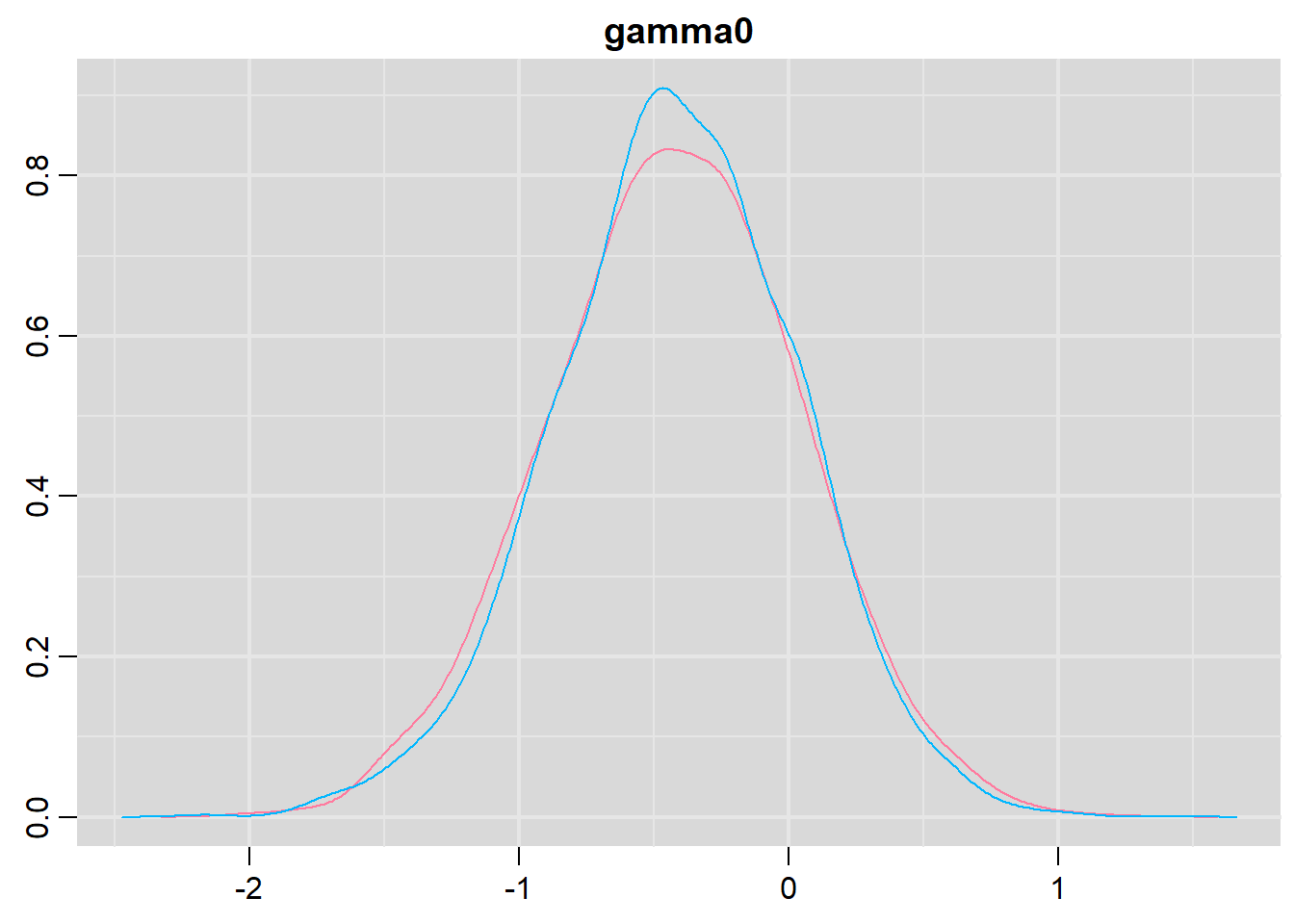
traplot(dat.zip.jags, parms = c('beta', 'gamma0'))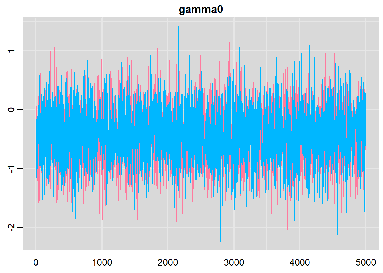
raftery.diag(as.mcmc(dat.zip.jags))NA [[1]]
NA
NA Quantile (q) = 0.025
NA Accuracy (r) = +/- 0.005
NA Probability (s) = 0.95
NA
NA Burn-in Total Lower bound Dependence
NA (M) (N) (Nmin) factor (I)
NA beta0 20 20276 3746 5.41
NA beta1 22 24038 3746 6.42
NA deviance 4 4636 3746 1.24
NA gamma0 5 5908 3746 1.58
NA theta 5 5908 3746 1.58
NA
NA
NA [[2]]
NA
NA Quantile (q) = 0.025
NA Accuracy (r) = +/- 0.005
NA Probability (s) = 0.95
NA
NA Burn-in Total Lower bound Dependence
NA (M) (N) (Nmin) factor (I)
NA beta0 20 21336 3746 5.70
NA beta1 20 22636 3746 6.04
NA deviance 3 4267 3746 1.14
NA gamma0 5 6078 3746 1.62
NA theta 5 6078 3746 1.62autocorr.diag(as.mcmc(dat.zip.jags))NA beta0 beta1 deviance gamma0 theta
NA Lag 0 1.00000000 1.00000000 1.00000000 1.000000000 1.000000000
NA Lag 1 0.88627108 0.88426590 0.51799594 0.232408997 0.227686735
NA Lag 5 0.58998005 0.59775827 0.19471855 0.002321179 0.001571686
NA Lag 10 0.35846288 0.35888205 0.06697926 0.017561785 0.015598223
NA Lag 50 -0.01753582 -0.01936659 -0.01212528 0.022040872 0.021016755Goodness of fit
#extract the samples for the two model parameters
coefs <- dat.zip.jags$BUGSoutput$sims.matrix[,1:2]
theta <- dat.zip.jags$BUGSoutput$sims.matrix[,'theta']
Xmat <- model.matrix(~x, data=dat.zip)
#expected values on a log scale
lambda<-coefs %*% t(Xmat)
#expected value on response scale
eta <- exp(lambda)
expY <- sweep(eta,1,(1-theta),"*")
varY <- eta+sweep(eta^2,1,theta,"*")
varY <- sweep(varY,1,(1-theta),'*')
#sweep across rows and then divide by lambda
Resid <- -1*sweep(expY,2,dat.zip$y,'-')/sqrt(varY)
#plot residuals vs expected values
plot(apply(Resid,2,mean)~apply(eta,2,mean))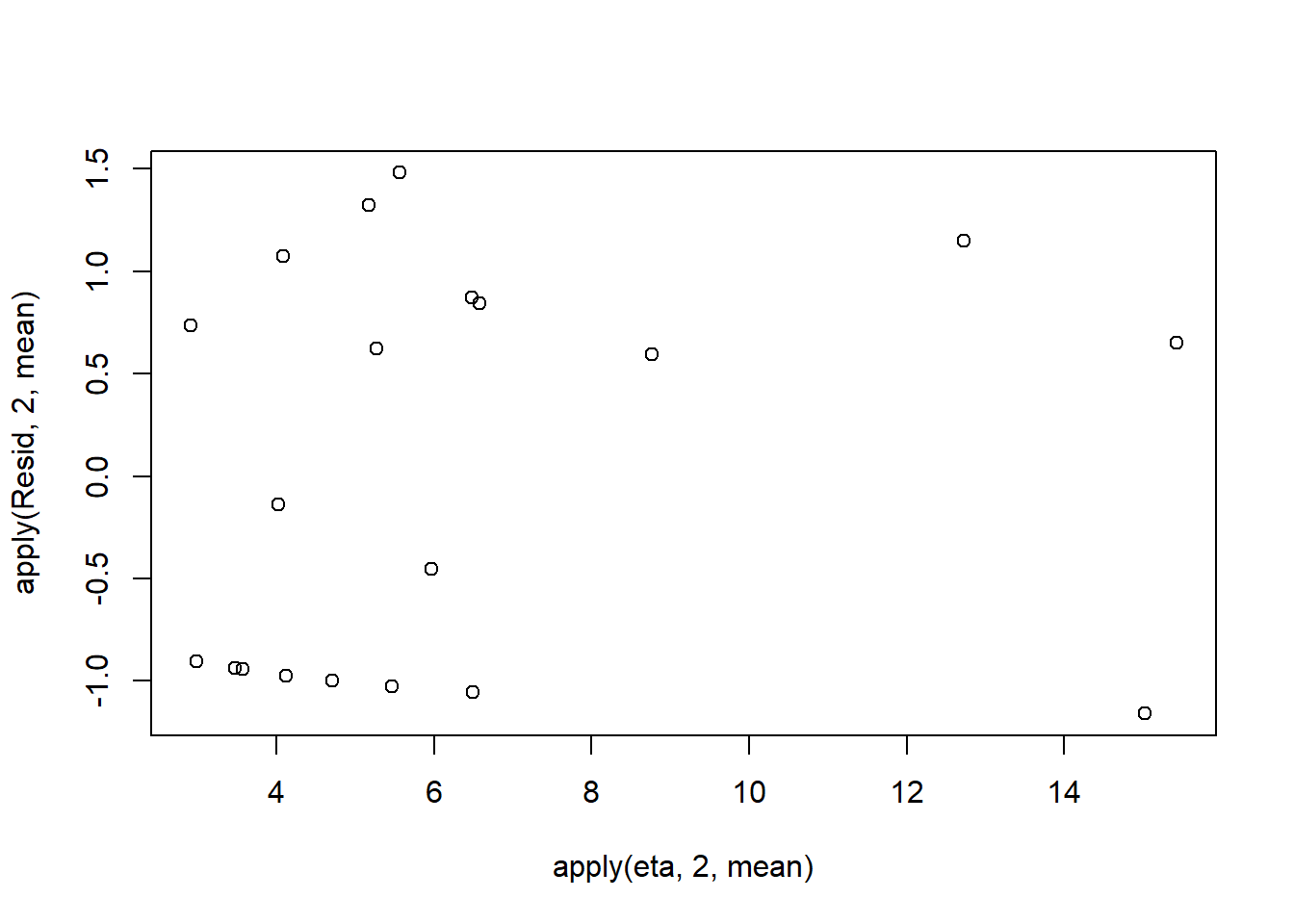
Now we will compare the sum of squared residuals to the sum of squares residuals that would be expected from a Poisson distribution matching that estimated by the model. Essentially this is estimating how well the Poisson distribution, the log-link function and the linear model approximates the observed data. When doing so, we need to consider the expected value and variance of the zero-inflated poisson.
SSres<-apply(Resid^2,1,sum, na.rm=T)

#generate a matrix of draws from a zero-inflated poisson (ZIP) distribution
# the matrix is the same dimensions as lambda
library(gamlss.dist)
#YNew <- matrix(rZIP(length(lambda),eta, theta),nrow=nrow(lambda))
lambda <- sweep(eta,1,ifelse(dat.zip$y==0,0,1),'*')
YNew <- matrix(rpois(length(lambda),lambda),nrow=nrow(lambda))
Resid1<-(expY - YNew)/sqrt(varY)
SSres.sim<-apply(Resid1^2,1,sum)
mean(SSres.sim>SSres, na.rm = T)
NA [1] 0.5619Since it is difficult to diagnose many issues from the typical residuals we will now explore simulated residuals.
#extract the samples for the two model parameters
coefs <- dat.zip.jags$BUGSoutput$sims.matrix[,1:2]
theta <- dat.zip.jags$BUGSoutput$sims.matrix[,'theta']
Xmat <- model.matrix(~x, data=dat.zip)
#expected values on a log scale
eta<-coefs %*% t(Xmat)
#expected value on response scale
lambda <- exp(eta)

simRes <- function(lambda, data,n=250, plot=T, family='negbin', size=NULL,theta=NULL) {
 require(gap)
 N = nrow(data)
 sim = switch(family,
    'poisson' = matrix(rpois(n*N,apply(lambda,2,mean)),ncol=N, byrow=TRUE),
    'negbin' = matrix(MASS:::rnegbin(n*N,apply(lambda,2,mean),size),ncol=N, byrow=TRUE),
        'zip' = matrix(gamlss.dist:::rZIP(n*N,apply(lambda,2,mean),theta),ncol=N, byrow=TRUE)
 )
 a = apply(sim + runif(n,-0.5,0.5),2,ecdf)
 resid<-NULL
 for (i in 1:nrow(data)) resid<-c(resid,a[[i]](data$y[i] + runif(1 ,-0.5,0.5)))
 if (plot==T) {
   par(mfrow=c(1,2))
   gap::qqunif(resid,pch = 2, bty = "n",
   logscale = F, col = "black", cex = 0.6, main = "QQ plot residuals",
   cex.main = 1, las=1)
   plot(resid~apply(lambda,2,mean), xlab='Predicted value', ylab='Standardized residual', las=1)
 }
 resid
}

simRes(lambda,dat.zip, family='zip',theta=theta)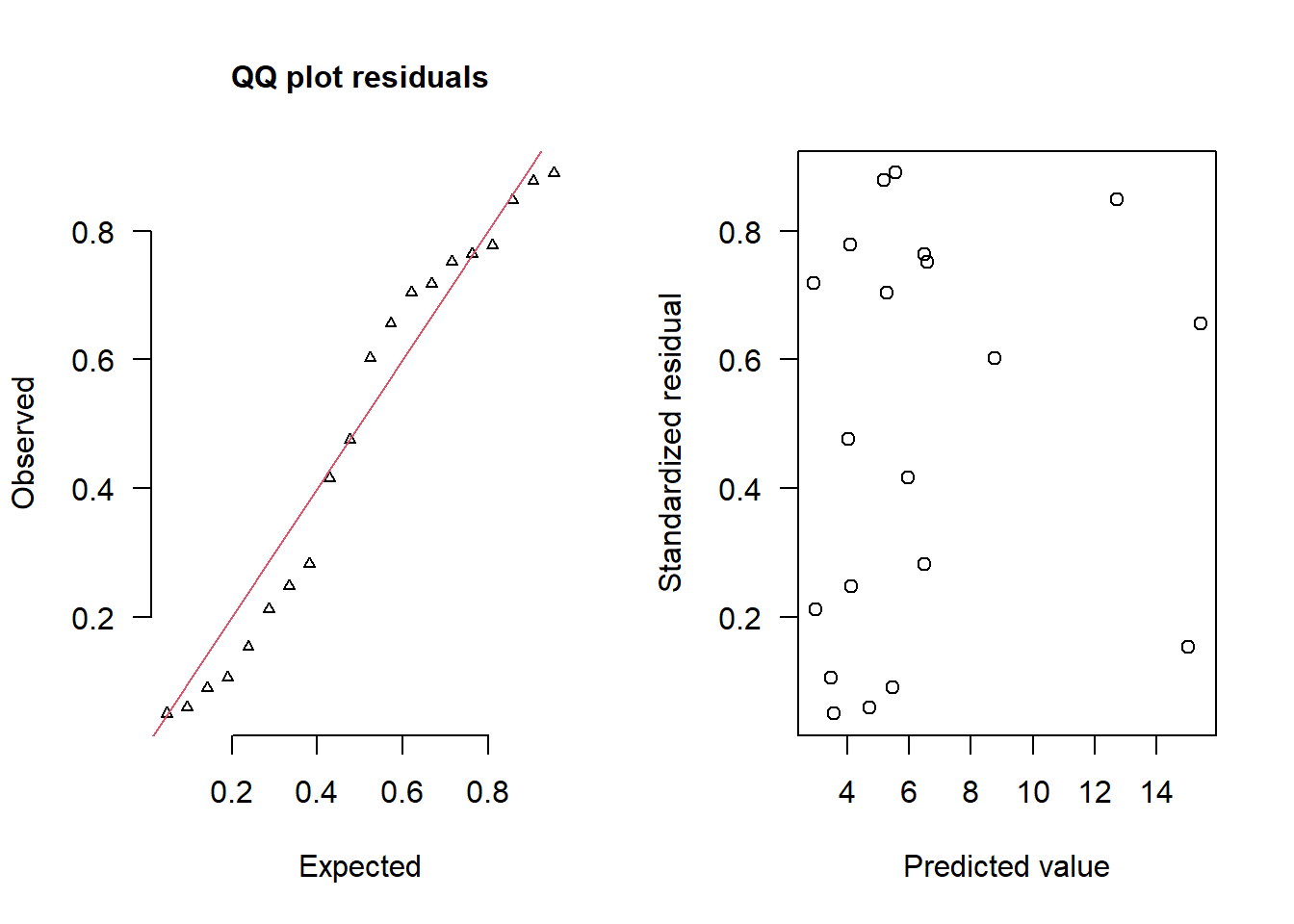
NA  [1] 0.718 0.212 0.106 0.050 0.476 0.778 0.248 0.060 0.878 0.704 0.090 0.890
NA [13] 0.416 0.764 0.282 0.752 0.602 0.848 0.154 0.656
The trend (black symbols) in the qq-plot does not appear to be overly non-linear (matching the ideal red line well), suggesting that the model is not overdispersed. The spread of standardized (simulated) residuals in the residual plot do not appear overly non-uniform. That is there is not trend in the residuals. Furthermore, there is not a concentration of points close to \(1\) or \(0\) (which would imply overdispersion). Hence, once zero-inflation is accounted for, the model does not display overdispersion. Although there is a slight hint of non-linearity in that the residuals are high for low and high fitted values and lower in the middle, this might well be an artifact of the small data set size. By change, most of the observed values in the middle range of the predictor were zero.
Exploring the model parameters
If there was any evidence that the assumptions had been violated or the model was not an appropriate fit, then we would need to reconsider the model and start the process again. In this case, there is no evidence that the test will be unreliable so we can proceed to explore the test statistics. As with most Bayesian models, it is best to base conclusions on medians rather than means.
print(dat.zip.jags)NA Inference for Bugs model at "modelzip.txt", fit using jags,
NA 2 chains, each with 10000 iterations (first 5000 discarded)
NA n.sims = 10000 iterations saved
NA mu.vect sd.vect 2.5% 25% 50% 75% 97.5% Rhat n.eff
NA beta0 0.930 0.282 0.365 0.742 0.933 1.128 1.468 1.003 860
NA beta1 0.090 0.021 0.049 0.076 0.090 0.104 0.132 1.002 1400
NA gamma0 -0.420 0.458 -1.349 -0.722 -0.417 -0.110 0.459 1.001 10000
NA theta 0.401 0.105 0.206 0.327 0.397 0.472 0.613 1.001 7600
NA deviance 80.674 2.501 77.856 78.867 80.008 81.801 87.064 1.001 10000
NA
NA For each parameter, n.eff is a crude measure of effective sample size,
NA and Rhat is the potential scale reduction factor (at convergence, Rhat=1).
NA
NA DIC info (using the rule, pD = var(deviance)/2)
NA pD = 3.1 and DIC = 83.8
NA DIC is an estimate of expected predictive error (lower deviance is better).adply(dat.zip.jags$BUGSoutput$sims.matrix, 2, function(x) {
data.frame(Median=median(x), Mean=mean(x), HPDinterval(as.mcmc(x)), HPDinterval(as.mcmc(x),p=0.5))
})NA X1 Median Mean lower upper lower.1
NA 1 beta0 0.93334635 0.92997411 0.37821529 1.4774189 0.7530788
NA 2 beta1 0.09005537 0.09005981 0.04864163 0.1313802 0.0749821
NA 3 deviance 80.00841187 80.67383245 77.63946567 85.5798539 77.8273778
NA 4 gamma0 -0.41667356 -0.41996110 -1.34903991 0.4586909 -0.7013225
NA 5 theta 0.39731301 0.40136809 0.19516803 0.6012233 0.3173026
NA upper.1
NA 1 1.13629442
NA 2 0.10333030
NA 3 80.10544007
NA 4 -0.09258569
NA 5 0.46170971#on original scale
adply(exp(dat.zip.jags$BUGSoutput$sims.matrix[,1:2]), 2, function(x) {
data.frame(Median=median(x), Mean=mean(x), HPDinterval(as.mcmc(x)), HPDinterval(as.mcmc(x),p=0.5))
})NA X1 Median Mean lower upper lower.1 upper.1
NA 1 beta0 2.543005 2.636434 1.280362 4.056990 1.911083 2.853498
NA 2 beta1 1.094235 1.094483 1.049844 1.140401 1.077865 1.108858Conclusions: We would reject the null hypothesis of no effect of \(x\) on \(y\). An increase in \(x\) is associated with a significant linear increase (positive slope) in the abundance of \(y\). Every \(1\) unit increase in \(x\) results in a log \(0.09\) unit increase in \(y\). We usually express this in terms of abundance rather than log abundance, so every \(1\) unit increase in \(x\) results in a (\(e^{0.09}=1.1\)) \(1.1\) unit increase in the abundance of \(y\).
Explorations of the trends
A measure of the strength of the relationship can be obtained according to:
\[ R^2 = 1 - \frac{\text{RSS}_{model}}{\text{RSS}_{null}} \]
Alternatively, we could use McFadden’s psuedo
\[ R^2 = 1- \frac{LL(Model_{full})}{LL(Model_{reduced}} \]
Xmat <- model.matrix(~x, dat=dat.zip)
#expected values on a log scale
neta<-coefs %*% t(Xmat)
#expected value on response scale
eta <- exp(neta)
lambda <- sweep(eta,2,ifelse(dat.zip$y==0,0,1),'*')
theta <- dat.zip.jags$BUGSoutput$sims.matrix[,'theta']
expY <- sweep(lambda,2,1-theta,'*')
#calculate the raw SS residuals
SSres <- apply((-1*(sweep(expY,2,dat.zip$y,'-')))^2,1,sum)
mean(SSres)
NA [1] 168.3814SSres.null <- sum((dat.zip$y - mean(dat.zip$y))^2)
#calculate the model r2
1-mean(SSres)/SSres.nullNA [1] 0.5977029Conclusions: \(50\)% of the variation in \(y\) abundance can be explained by its relationship with \(x\). Finally, we will create a summary plot.
par(mar = c(4, 5, 0, 0))
plot(y ~ x, data = dat.zip, type = "n", ann = F, axes = F)
points(y ~ x, data = dat.zip, pch = 16)
xs <- seq(min(dat.zip$x,na.rm=TRUE),max(dat.zip$x,na.rm=TRUE), l = 1000)
Xmat <- model.matrix(~xs)
eta<-coefs %*% t(Xmat)
ys <- exp(eta)
library(plyr)
library(coda)
data.tab <- adply(ys,2,function(x) {
  data.frame(Median=median(x), HPDinterval(as.mcmc(x)))
})
data.tab <- cbind(x=xs,data.tab)
points(Median ~ x, data=data.tab,col = "black", type = "l")
lines(lower ~ x, data=data.tab,col = "black", type = "l", lty = 2)
lines(upper ~ x, data=data.tab,col = "black", type = "l", lty = 2)

axis(1)
mtext("X", 1, cex = 1.5, line = 3)
axis(2, las = 2)
mtext("Abundance of Y", 2, cex = 1.5, line = 3)
box(bty = "l")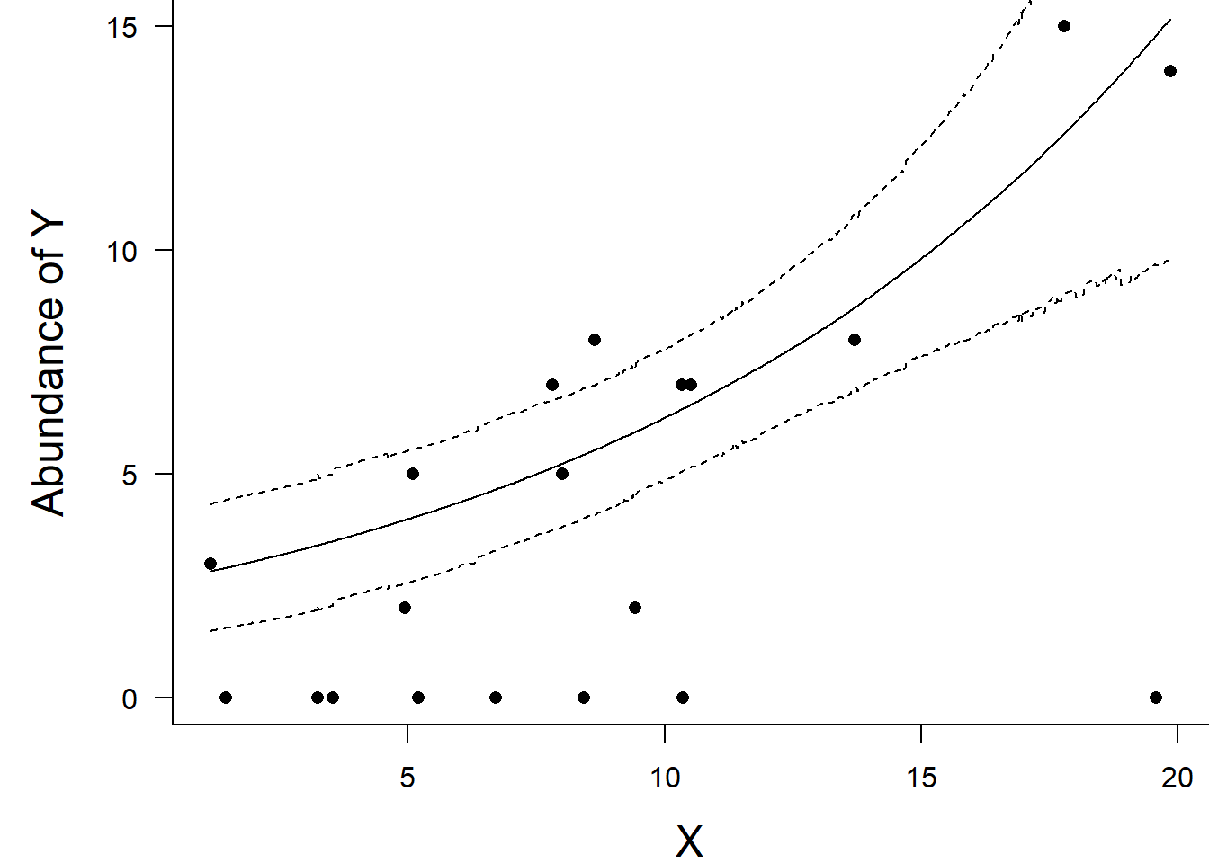
Full log-likelihood function
Now lets try it by specifying log-likelihood and the zero trick. When applying this trick, we need to manually calculate the deviance as the inbuilt deviance will be based on the log-likelihood of estimating the zeros (as part of the zero trick) rather than the deviance of the intended model. The one advantage of the zero trick is that the Deviance and thus DIC, AIC provided by R2jags will be incorrect. Hence, they too need to be manually defined within JAGS I suspect that the AIC calculation I have used is incorrect.
Xmat <- model.matrix(~x, dat.zip)
nX <- ncol(Xmat)
dat.zip.list2 <- with(dat.zip,list(Y=y, X=Xmat,N=nrow(dat.zip), mu=rep(0,nX),
                  Sigma=diag(1.0E-06,nX), zeros=rep(0,nrow(dat)), C=10000))
modelString="
model {
  for (i in 1:N) {
     zeros[i] ~ dpois(zeros.lambda[i])
     zeros.lambda[i] <- -ll[i] + C
     ll[i] <- Y[i]*log(lambda[i]) - lambda[i] - loggam(Y[i]+1)
     eta[i] <- inprod(beta[], X[i,])
     log(lambda[i]) <- eta[i]
    llm[i] <- Y[i]*log(meanlambda) - meanlambda - loggam(Y[i]+1)
  }
  meanlambda <- mean(lambda)
  beta ~ dmnorm(mu[],Sigma[,])
  dev <- sum(-2*ll)
  pD <- mean(dev)-sum(-2*llm)
  AIC <- min(dev+(2*pD))
}
"

writeLines(modelString, con='modelzip_ll.txt')

params <- c('beta','dev','AIC')
nChains = 2
burnInSteps = 5000
thinSteps = 1
numSavedSteps = 20000
nIter = ceiling((numSavedSteps * thinSteps)/nChains)

dat.ZIP.jags3  <- jags(data=dat.zip.list2,model.file='modelzip_ll.txt', param=params,
                   n.chains=nChains, n.iter=nIter, n.burnin=burnInSteps, n.thin=thinSteps)
NA Compiling model graph
NA Resolving undeclared variables
NA Allocating nodes
NA Graph information:
NA Observed stochastic nodes: 20
NA Unobserved stochastic nodes: 1
NA Total graph size: 328
NA
NA Initializing modelprint(dat.ZIP.jags3 )NA Inference for Bugs model at "modelzip_ll.txt", fit using jags,
NA 2 chains, each with 10000 iterations (first 5000 discarded)
NA n.sims = 10000 iterations saved
NA mu.vect sd.vect 2.5% 25% 50% 75%
NA AIC 61.488 3.844 57.991 58.846 60.144 62.785
NA beta[1] 0.329 0.225 -0.122 0.176 0.331 0.475
NA beta[2] 0.104 0.017 0.070 0.093 0.104 0.116
NA dev 124.472 1.801 122.700 123.170 123.871 125.221
NA deviance 400124.472 1.801 400122.700 400123.170 400123.871 400125.221
NA 97.5% Rhat n.eff
NA AIC 72.257 1.089 35
NA beta[1] 0.785 1.071 67
NA beta[2] 0.137 1.051 69
NA dev 129.054 1.042 53
NA deviance 400129.054 1.000 1
NA
NA For each parameter, n.eff is a crude measure of effective sample size,
NA and Rhat is the potential scale reduction factor (at convergence, Rhat=1).
NA
NA DIC info (using the rule, pD = var(deviance)/2)
NA pD = 1.6 and DIC = 400126.1
NA DIC is an estimate of expected predictive error (lower deviance is better).Zero inflated Negative Binomial
Data generation
Lets say we wanted to model the abundance of an item (\(y\)) against a continuous predictor (\(x\)). As this section is mainly about the generation of artificial data (and not specifically about what to do with the data), understanding the actual details are optional and can be safely skipped.
set.seed(37) #34.5  #4 #10 #16 #17 #26
#The number of samples
n.x <- 20
#Create x values that at uniformly distributed throughout the rate of 1 to 20
x <- sort(runif(n = n.x, min = 1, max =20))
mm <- model.matrix(~x)
intercept <- 0.6
slope=0.1
#The linear predictor
linpred <- mm %*% c(intercept,slope)
#Predicted y values
lambda <- exp(linpred)
#Add some noise and make binomial
library(gamlss.dist)
library(MASS)
#fixed latent binomial
y<- rZINBI(n.x,lambda, 0.4)
#latent binomial influenced by the linear predictor
#y<- rZINB(n.x,lambda, 1-exp(linpred)/(1+exp(linpred)))
dat.zinb <- data.frame(y,x)

summary(dat.glm.nb<-glm.nb(y~x, dat.zinb))
NA
NA Call:
NA glm.nb(formula = y ~ x, data = dat.zinb, init.theta = 0.4646673144,
NA link = log)
NA
NA Coefficients:
NA Estimate Std. Error z value Pr(>|z|)
NA (Intercept) 0.914191 0.796804 1.147 0.251
NA x 0.009149 0.067713 0.135 0.893
NA
NA (Dispersion parameter for Negative Binomial(0.4647) family taken to be 1)
NA
NA Null deviance: 20.303 on 19 degrees of freedom
NA Residual deviance: 20.282 on 18 degrees of freedom
NA AIC: 90.365
NA
NA Number of Fisher Scoring iterations: 1
NA
NA
NA Theta: 0.465
NA Std. Err.: 0.218
NA
NA 2 x log-likelihood: -84.365plot(glm.nb(y~x, dat.zinb))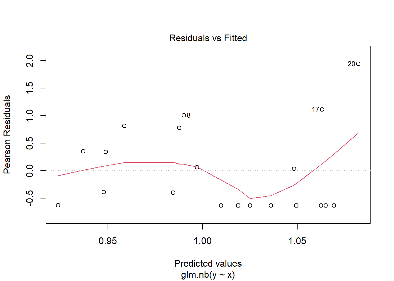
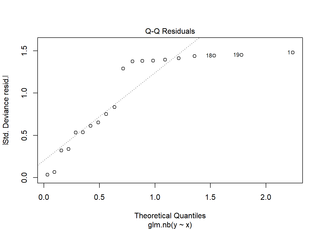
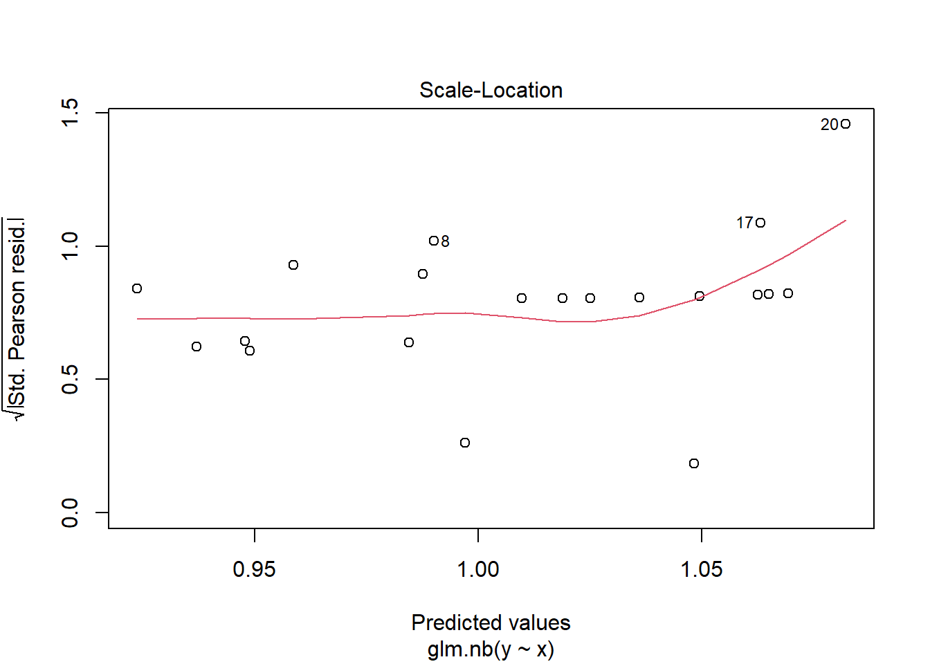
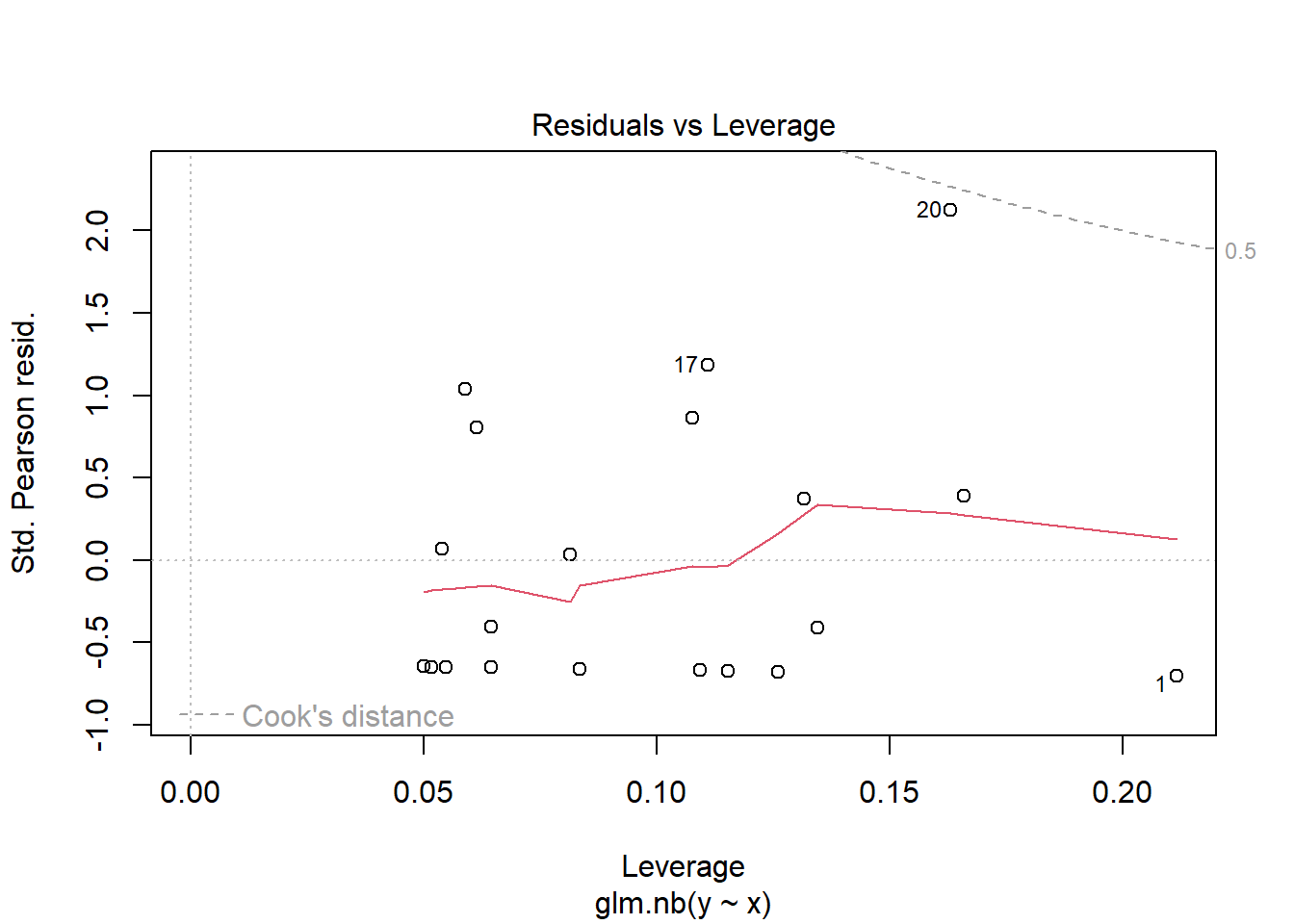
library(pscl)
summary(dat.zeroinfl<-zeroinfl(y ~ x | 1, dist = "negbin", data = dat.zinb))
NA
NA Call:
NA zeroinfl(formula = y ~ x | 1, data = dat.zinb, dist = "negbin")
NA
NA Pearson residuals:
NA Min 1Q Median 3Q Max
NA -0.9609 -0.9268 -0.4446 1.0425 1.7556
NA
NA Count model coefficients (negbin with log link):
NA Estimate Std. Error z value Pr(>|z|)
NA (Intercept) 0.92733 0.32507 2.853 0.00433 **
NA x 0.06870 0.02755 2.494 0.01263 *
NA Log(theta) 3.36066 3.59739 0.934 0.35020
NA
NA Zero-inflation model coefficients (binomial with logit link):
NA Estimate Std. Error z value Pr(>|z|)
NA (Intercept) -0.2250 0.4559 -0.494 0.622
NA ---
NA Signif. codes: 0 '***' 0.001 '**' 0.01 '*' 0.05 '.' 0.1 ' ' 1
NA
NA Theta = 28.8082
NA Number of iterations in BFGS optimization: 17
NA Log-likelihood: -38.54 on 4 Dfplot(resid(zeroinfl(y ~ x | 1, dist = "negbin", data = dat.zinb))~fitted(zeroinfl(y ~ x | 1, dist = "negbin")))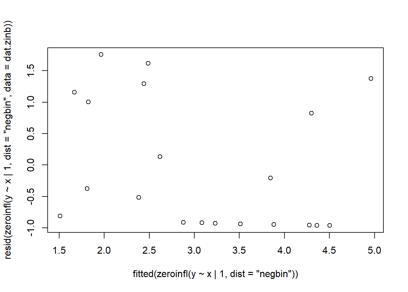
vuong(dat.glm.nb, dat.zeroinfl)NA Vuong Non-Nested Hypothesis Test-Statistic:
NA (test-statistic is asymptotically distributed N(0,1) under the
NA null that the models are indistinguishible)
NA -------------------------------------------------------------
NA Vuong z-statistic H_A p-value
NA Raw -1.2809521 model2 > model1 0.10011
NA AIC-corrected -0.9296587 model2 > model1 0.17627
NA BIC-corrected -0.7547616 model2 > model1 0.22520library(gamlss)
summary(gamlss(y~x, data=dat.zinb, family='ZINBI'))NA GAMLSS-RS iteration 1: Global Deviance = 82.35
NA GAMLSS-RS iteration 2: Global Deviance = 82.0176
NA GAMLSS-RS iteration 3: Global Deviance = 81.8115
NA GAMLSS-RS iteration 4: Global Deviance = 81.6241
NA GAMLSS-RS iteration 5: Global Deviance = 81.5175
NA GAMLSS-RS iteration 6: Global Deviance = 81.5429
NA GAMLSS-RS iteration 7: Global Deviance = 81.6384
NA GAMLSS-RS iteration 8: Global Deviance = 81.6956
NA GAMLSS-RS iteration 9: Global Deviance = 81.702
NA GAMLSS-RS iteration 10: Global Deviance = 81.6899
NA GAMLSS-RS iteration 11: Global Deviance = 81.644
NA GAMLSS-RS iteration 12: Global Deviance = 81.4995
NA GAMLSS-RS iteration 13: Global Deviance = 81.4366
NA GAMLSS-RS iteration 14: Global Deviance = 81.4913
NA GAMLSS-RS iteration 15: Global Deviance = 81.583
NA GAMLSS-RS iteration 16: Global Deviance = 81.6803
NA GAMLSS-RS iteration 17: Global Deviance = 81.7197
NA GAMLSS-RS iteration 18: Global Deviance = 81.7177
NA GAMLSS-RS iteration 19: Global Deviance = 81.6711
NA GAMLSS-RS iteration 20: Global Deviance = 81.5165
NA ******************************************************************
NA Family: c("ZINBI", "Zero inflated negative binomial type I")
NA
NA Call: gamlss(formula = y ~ x, family = "ZINBI", data = dat.zinb)
NA
NA Fitting method: RS()
NA
NA ------------------------------------------------------------------
NA Mu link function: log
NA Mu Coefficients:
NA Estimate Std. Error t value Pr(>|t|)
NA (Intercept) 0.94930 0.93174 1.019 0.322
NA x 0.03794 0.07030 0.540 0.596
NA
NA ------------------------------------------------------------------
NA Sigma link function: log
NA Sigma Coefficients:
NA Estimate Std. Error t value Pr(>|t|)
NA (Intercept) -0.2866 0.7254 -0.395 0.697
NA
NA ------------------------------------------------------------------
NA Nu link function: logit
NA Nu Coefficients:
NA Estimate Std. Error t value Pr(>|t|)
NA (Intercept) -0.8664 0.6832 -1.268 0.22
NA
NA ------------------------------------------------------------------
NA No. of observations in the fit: 20
NA Degrees of Freedom for the fit: 4
NA Residual Deg. of Freedom: 16
NA at cycle: 20
NA
NA Global Deviance: 81.51652
NA AIC: 89.51652
NA SBC: 93.49945
NA ******************************************************************summary(gamlss(y~x, nu.fo=y~x,data=dat.zinb, family='ZINBI'))NA GAMLSS-RS iteration 1: Global Deviance = 79.3063
NA GAMLSS-RS iteration 2: Global Deviance = 77.6325
NA GAMLSS-RS iteration 3: Global Deviance = 77.4263
NA GAMLSS-RS iteration 4: Global Deviance = 77.1265
NA GAMLSS-RS iteration 5: Global Deviance = 77.0111
NA GAMLSS-RS iteration 6: Global Deviance = 76.9765
NA GAMLSS-RS iteration 7: Global Deviance = 76.9662
NA GAMLSS-RS iteration 8: Global Deviance = 76.9626
NA GAMLSS-RS iteration 9: Global Deviance = 76.9583
NA GAMLSS-RS iteration 10: Global Deviance = 76.9579
NA ******************************************************************
NA Family: c("ZINBI", "Zero inflated negative binomial type I")
NA
NA Call: gamlss(formula = y ~ x, nu.formula = y ~ x, family = "ZINBI",
NA data = dat.zinb)
NA
NA Fitting method: RS()
NA
NA ------------------------------------------------------------------
NA Mu link function: log
NA Mu Coefficients:
NA Estimate Std. Error t value Pr(>|t|)
NA (Intercept) 0.80319 0.49858 1.611 0.128
NA x 0.05928 0.05851 1.013 0.327
NA
NA ------------------------------------------------------------------
NA Sigma link function: log
NA Sigma Coefficients:
NA Estimate Std. Error t value Pr(>|t|)
NA (Intercept) -0.6147 1.8864 -0.326 0.749
NA
NA ------------------------------------------------------------------
NA Nu link function: logit
NA Nu Coefficients:
NA Estimate Std. Error t value Pr(>|t|)
NA (Intercept) -3.4494 2.7228 -1.267 0.225
NA x 0.2298 0.1700 1.352 0.196
NA
NA ------------------------------------------------------------------
NA No. of observations in the fit: 20
NA Degrees of Freedom for the fit: 5
NA Residual Deg. of Freedom: 15
NA at cycle: 10
NA
NA Global Deviance: 76.95789
NA AIC: 86.95789
NA SBC: 91.93655
NA ******************************************************************Exploratory data analysis
Check the distribution of the \(y\) abundances.
hist(dat.zinb$y)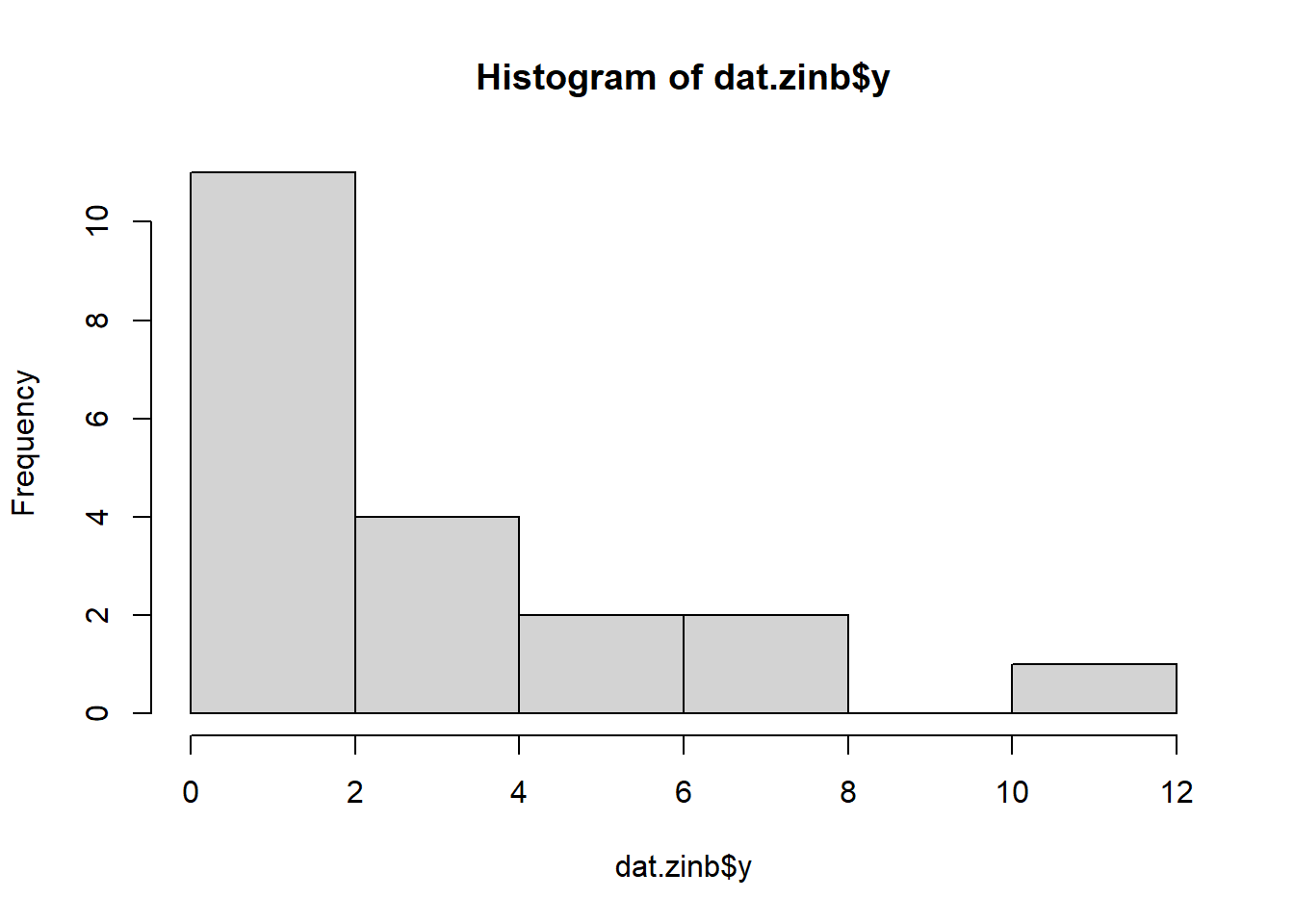
boxplot(dat.zinb$y, horizontal=TRUE)
rug(jitter(dat.zinb$y))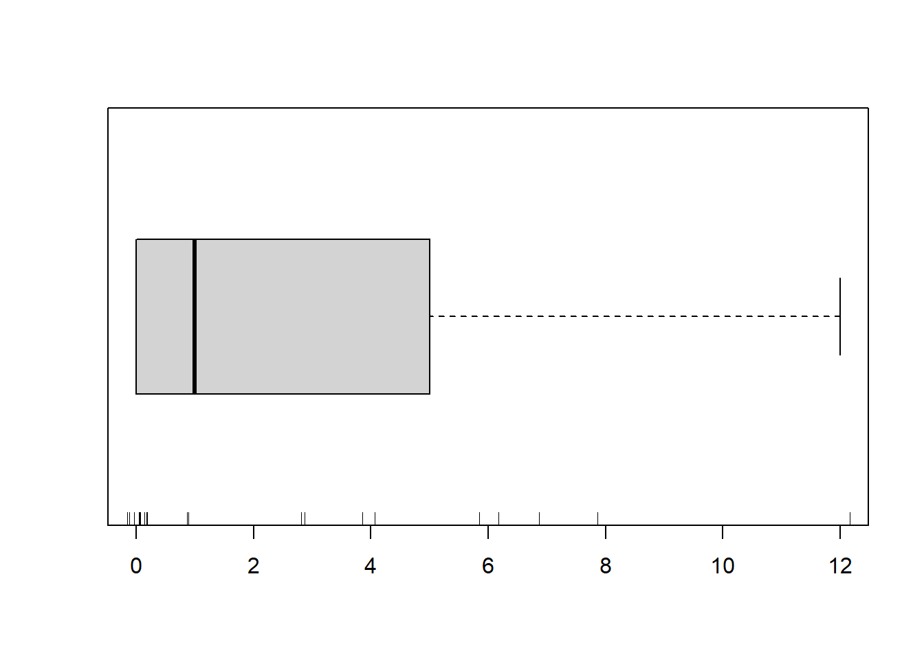
There is definitely signs of non-normality that would warrant Poisson or negative binomial models. Further to that, there appears to be a large number of zeros and a possible clumpiness that are likely to be the cause of overdispersion A zero-inflated negative binomial model is likely to be one of the most effective for modeling these data. Lets now explore linearity by creating a histogram of the predictor variable (\(x\)). Note, it is difficult to directly assess issues of linearity. Indeed, a scatterplot with lowess smoother will be largely influenced by the presence of zeros. One possible way of doing so is to explore the trend in the non-zero data.
hist(dat.zinb$x)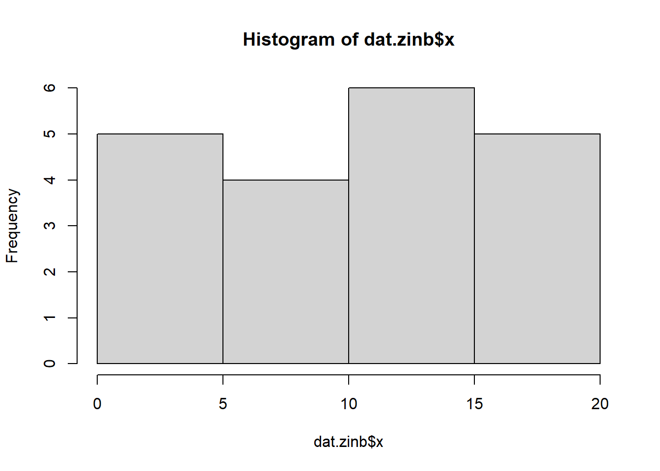
#now for the scatterplot
plot(y~x, dat.zinb, log="y")
with(subset(dat.zinb,y>0), lines(lowess(y~x)))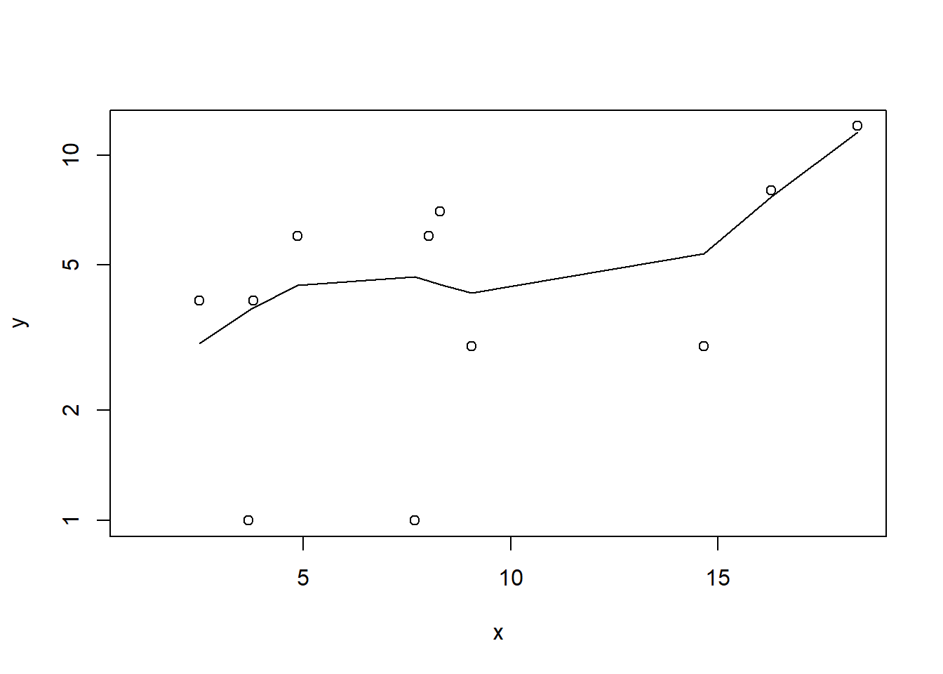
Conclusions: the predictor (\(x\)) does not display any skewness or other issues that might lead to non-linearity. The lowess smoother on the non-zero data cloud does not display major deviations from a straight line and thus linearity is likely to be satisfied. Violations of linearity (whilst difficult to be certain about due to the unknown influence of the zeros) could be addressed by either:
define a non-linear linear predictor (such as a polynomial, spline or other non-linear function).
transform the scale of the predictor variables.
Although we have already established that there are few zeros in the data (and thus overdispersion is unlikely to be an issue), we can also explore this by comparing the number of zeros in the data to the number of zeros that would be expected from a Poisson distribution with a mean equal to the mean count of the data.
#proportion of 0's in the data
dat.zinb.tab<-table(dat.zinb$y==0)
dat.zinb.tab/sum(dat.zinb.tab)
NA
NA FALSE TRUE
NA 0.55 0.45#proportion of 0's expected from a Poisson distribution
mu <- mean(dat.zinb$y)
v <- var(dat.zinb$y)
size <- mu + (mu^2)/v
cnts <- rnbinom(1000, mu=mu, size=size)
dat.zinb.tabE <- table(cnts == 0)
dat.zinb.tabE/sum(dat.zinb.tabE)NA
NA FALSE TRUE
NA 0.861 0.139In the above, the value under FALSE is the proportion of non-zero values in the data and the value under TRUE is the proportion of zeros in the data. In this example, the proportion of zeros observed (\(45\)%) far exceeds that that would have been expected (\(14\)%). Hence it is highly likely that any models will be zero-inflated.
Model fitting
\[ y_i \sim \text{ZINB}(\lambda_i, \theta), \]
where \(\text{logit}(\theta) = \gamma_0\), \(\log(\lambda_i)=\eta_i\), with \(\eta_i=\beta_0+\beta_1x_{i}\) and \(\beta_0,\beta_1,\gamma_0 \sim N(0, 10000)\).
dat.zinb.list <- with(dat.zinb,list(Y=y, X=x,N=nrow(dat.zinb),z=ifelse(y==0,0,1)))
modelString="
model {
  for (i in 1:N) {
     z[i] ~ dbern(psi.min)
     Y[i] ~ dnegbin(p[i],size)
     p[i] <- size/(size+mu.eff[i])
     mu.eff[i] <- z[i]*mu[i]
     eta[i] <- beta0 + beta1*X[i]
     log(mu[i]) <- eta[i]
  }
  gamma ~ dnorm(0,0.001)
  psi.min <- min(0.9999, max(0.00001, (1-psi)))
  logit(psi) <- max(-20, min(20, gamma))
  size ~ dunif(0.001, 5)
  theta <- pow(1/mean(p),2)
  beta0 ~ dnorm(0,1.0E-06)
  beta1 ~ dnorm(0,1.0E-06)
}
"
writeLines(modelString, con='modelzinb.txt')

params <- c('beta0','beta1', 'size', 'theta')
nChains = 2
burnInSteps = 5000
thinSteps = 1
numSavedSteps = 20000
nIter = ceiling((numSavedSteps * thinSteps)/nChains)

dat.zinb.jags <- jags(data=dat.zinb.list,model.file='modelzinb.txt', param=params,
                   n.chains=nChains, n.iter=nIter, n.burnin=burnInSteps, n.thin=thinSteps)
NA Compiling model graph
NA Resolving undeclared variables
NA Allocating nodes
NA Graph information:
NA Observed stochastic nodes: 40
NA Unobserved stochastic nodes: 4
NA Total graph size: 205
NA
NA Initializing modelprint(dat.zinb.jags)NA Inference for Bugs model at "modelzinb.txt", fit using jags,
NA 2 chains, each with 10000 iterations (first 5000 discarded)
NA n.sims = 10000 iterations saved
NA mu.vect sd.vect 2.5% 25% 50% 75% 97.5% Rhat n.eff
NA beta0 0.971 0.460 0.055 0.678 0.963 1.273 1.868 1.007 250
NA beta1 0.067 0.042 -0.016 0.039 0.066 0.094 0.151 1.008 200
NA size 3.501 1.015 1.389 2.763 3.644 4.351 4.935 1.001 10000
NA theta 2.200 0.367 1.721 1.937 2.115 2.371 3.145 1.001 3300
NA deviance 82.769 2.843 79.139 80.663 82.139 84.254 89.891 1.001 10000
NA
NA For each parameter, n.eff is a crude measure of effective sample size,
NA and Rhat is the potential scale reduction factor (at convergence, Rhat=1).
NA
NA DIC info (using the rule, pD = var(deviance)/2)
NA pD = 4.0 and DIC = 86.8
NA DIC is an estimate of expected predictive error (lower deviance is better).Model evaluation
denplot(dat.zinb.jags, parms = c('beta0','beta1', 'size', 'theta'))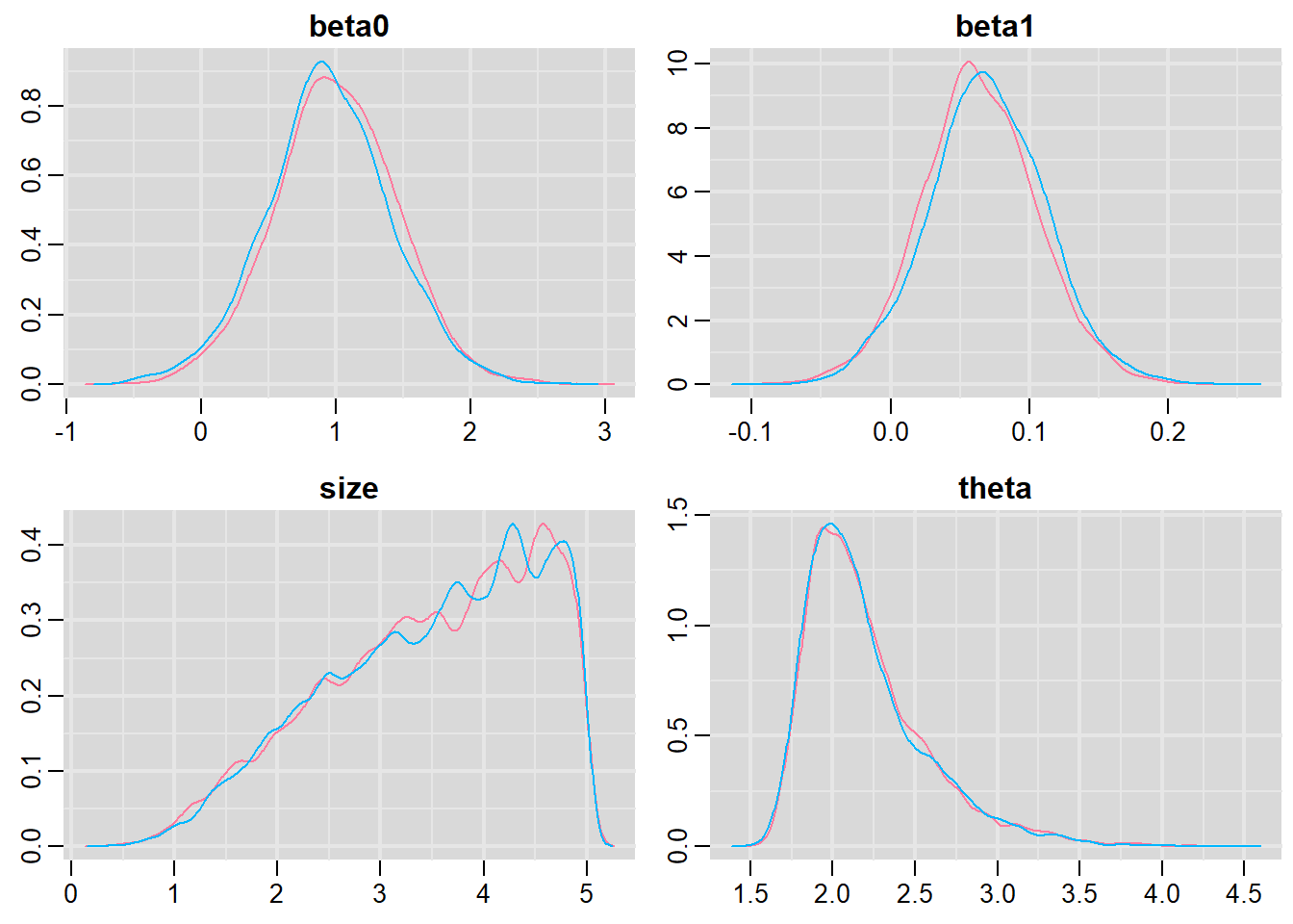
traplot(dat.zinb.jags, parms = c('beta0','beta1', 'size', 'theta'))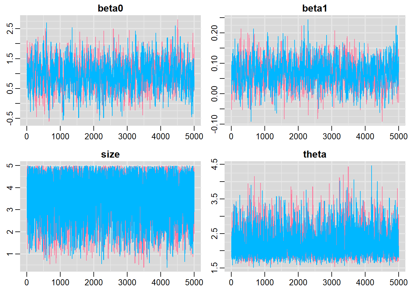
raftery.diag(as.mcmc(dat.zinb.jags))NA [[1]]
NA
NA Quantile (q) = 0.025
NA Accuracy (r) = +/- 0.005
NA Probability (s) = 0.95
NA
NA Burn-in Total Lower bound Dependence
NA (M) (N) (Nmin) factor (I)
NA beta0 15 16236 3746 4.33
NA beta1 14 15725 3746 4.20
NA deviance 3 4484 3746 1.20
NA size 5 5771 3746 1.54
NA theta 3 4338 3746 1.16
NA
NA
NA [[2]]
NA
NA Quantile (q) = 0.025
NA Accuracy (r) = +/- 0.005
NA Probability (s) = 0.95
NA
NA Burn-in Total Lower bound Dependence
NA (M) (N) (Nmin) factor (I)
NA beta0 27 27564 3746 7.36
NA beta1 18 21057 3746 5.62
NA deviance 3 4410 3746 1.18
NA size 5 5771 3746 1.54
NA theta 2 3995 3746 1.07autocorr.diag(as.mcmc(dat.zinb.jags))NA beta0 beta1 deviance size theta
NA Lag 0 1.00000000 1.00000000 1.00000000 1.000000000 1.000000000
NA Lag 1 0.82187294 0.82300377 0.55172222 0.391115803 0.387289605
NA Lag 5 0.44679310 0.44494849 0.13559995 0.045297725 0.067379632
NA Lag 10 0.19928140 0.20123773 0.05371302 0.008341721 0.013304093
NA Lag 50 -0.04037202 -0.04473554 -0.02496182 0.011474420 0.007333003Goodness of fit
#extract the samples for the two model parameters
coefs <- dat.zinb.jags$BUGSoutput$sims.matrix[,1:2]
theta <- dat.zinb.jags$BUGSoutput$sims.matrix[,'theta']
Xmat <- model.matrix(~x, data=dat.zinb)
#expected values on a log scale
lambda<-coefs %*% t(Xmat)
#expected value on response scale
eta <- exp(lambda)
expY <- sweep(eta,1,(1-theta),"*")
varY <- eta+sweep(eta^2,1,theta,"*")
head(varY)
NA 1 2 3 4 5 6 7 8
NA [1,] 10.844323 13.189501 15.47499 15.73287 18.21519 26.87133 28.14742 29.27065
NA [2,] 71.832694 61.952112 54.97632 54.30484 48.72535 36.70113 35.49495 34.51074
NA [3,] 24.764991 24.273552 23.88302 23.84316 23.49392 22.60135 22.49799 22.41131
NA [4,] 6.397443 8.786249 11.40150 11.71375 14.89149 28.26188 30.51610 32.55772
NA [5,] 27.048585 28.561484 29.85015 29.98628 31.21706 34.70423 35.14294 35.51685
NA [6,] 32.911549 36.163316 39.03708 39.34619 42.18864 50.70280 51.82155 52.78337
NA 9 10 11 12 13 14 15
NA [1,] 32.48606 39.45733 45.43874 50.02645 59.31437 71.66019 73.00520
NA [2,] 32.02933 27.89750 25.25717 23.61192 20.97369 18.40930 18.17586
NA [3,] 22.18262 21.76433 21.46712 21.26761 20.92017 20.54281 20.50616
NA [4,] 38.69312 53.42044 67.53693 79.24793 105.19992 144.10581 148.63604
NA [5,] 36.53055 38.49254 39.97741 41.01961 42.92731 45.14296 45.36660
NA [6,] 55.42928 60.70818 64.84042 67.81058 73.39529 80.11924 80.81199
NA 16 17 18 19 20
NA [1,] 89.37583 90.29710 93.03697 99.45044 121.73297
NA [2,] 15.83105 15.72115 15.40547 14.72560 12.85289
NA [3,] 20.11263 20.09293 20.03565 19.90863 19.52937
NA [4,] 208.15726 211.74132 222.54395 248.66128 348.12988
NA [5,] 47.86864 47.99890 48.38049 49.24196 51.94528
NA [6,] 88.73695 89.15824 90.39740 93.22189 102.32692#varY <- sweep(varY,1,(1-theta),'*')
#sweep across rows and then divide by lambda
Resid <- -1*sweep(expY,2,dat.zinb$y,'-')/sqrt(varY)
#plot residuals vs expected values
plot(apply(Resid,2,mean)~apply(eta,2,mean))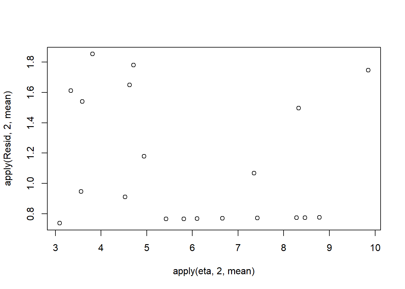
Now we will compare the sum of squared residuals to the sum of squares residuals that would be expected from a Poisson distribution matching that estimated by the model. Essentially this is estimating how well the Poisson distribution, the log-link function and the linear model approximates the observed data. When doing so, we need to consider the expected value and variance of the zero-inflated poisson.
SSres<-apply(Resid^2,1,sum, na.rm=T)

#generate a matrix of draws from a zero-inflated poisson (ZINB) distribution
# the matrix is the same dimensions as lambda
library(gamlss.dist)
#YNew <- matrix(rZINB(length(lambda),eta, theta),nrow=nrow(lambda))
lambda <- sweep(eta,1,ifelse(dat.zinb$y==0,0,1),'*')
YNew <- matrix(rpois(length(lambda),lambda),nrow=nrow(lambda))
Resid1<-(expY - YNew)/sqrt(varY)
SSres.sim<-apply(Resid1^2,1,sum)
mean(SSres.sim>SSres, na.rm = T)
NA [1] 0.5212Exploring the model parameters
If there was any evidence that the assumptions had been violated or the model was not an appropriate fit, then we would need to reconsider the model and start the process again. In this case, there is no evidence that the test will be unreliable so we can proceed to explore the test statistics. As with most Bayesian models, it is best to base conclusions on medians rather than means.
print(dat.zinb.jags)NA Inference for Bugs model at "modelzinb.txt", fit using jags,
NA 2 chains, each with 10000 iterations (first 5000 discarded)
NA n.sims = 10000 iterations saved
NA mu.vect sd.vect 2.5% 25% 50% 75% 97.5% Rhat n.eff
NA beta0 0.971 0.460 0.055 0.678 0.963 1.273 1.868 1.007 250
NA beta1 0.067 0.042 -0.016 0.039 0.066 0.094 0.151 1.008 200
NA size 3.501 1.015 1.389 2.763 3.644 4.351 4.935 1.001 10000
NA theta 2.200 0.367 1.721 1.937 2.115 2.371 3.145 1.001 3300
NA deviance 82.769 2.843 79.139 80.663 82.139 84.254 89.891 1.001 10000
NA
NA For each parameter, n.eff is a crude measure of effective sample size,
NA and Rhat is the potential scale reduction factor (at convergence, Rhat=1).
NA
NA DIC info (using the rule, pD = var(deviance)/2)
NA pD = 4.0 and DIC = 86.8
NA DIC is an estimate of expected predictive error (lower deviance is better).adply(dat.zinb.jags$BUGSoutput$sims.matrix, 2, function(x) {
data.frame(Median=median(x), Mean=mean(x), HPDinterval(as.mcmc(x)), HPDinterval(as.mcmc(x),p=0.5))
})NA X1 Median Mean lower upper lower.1
NA 1 beta0 0.96339931 0.97060322 0.05196655 1.8646388 0.68771701
NA 2 beta1 0.06565837 0.06658472 -0.01850221 0.1478933 0.03570031
NA 3 deviance 82.13938661 82.76912313 78.75619568 88.5891138 79.69050804
NA 4 size 3.64385931 3.50054311 1.63847682 4.9995959 3.62583688
NA 5 theta 2.11463918 2.19954948 1.65289052 2.9565781 1.83698278
NA upper.1
NA 1 1.28169341
NA 2 0.09027889
NA 3 82.76458253
NA 4 4.98121591
NA 5 2.20696839#on original scale
adply(exp(dat.zinb.jags$BUGSoutput$sims.matrix[,1:2]), 2, function(x) {
data.frame(Median=median(x), Mean=mean(x), HPDinterval(as.mcmc(x)), HPDinterval(as.mcmc(x),p=0.5))
})NA X1 Median Mean lower upper lower.1 upper.1
NA 1 beta0 2.620590 2.935935 0.7910564 5.701997 1.628127 3.096623
NA 2 beta1 1.067862 1.069796 0.9816679 1.159389 1.036345 1.094479Conclusions: We would reject the null hypothesis of no effect of \(x\) on \(y\). An increase in \(x\) is associated with a significant linear increase (positive slope) in the abundance of \(y\). Every \(1\) unit increase in \(x\) results in a log \(0.06\) unit increase in \(y\). We usually express this in terms of abundance rather than log abundance, so every \(1\) unit increase in \(x\) results in a (\(e^{0.06}=1.07\)) \(1.07\) unit increase in the abundance of \(y\).
References
Plummer, Martyn. 2004. “JAGS: Just Another Gibbs Sampler.”
Su, Yu-Sung, Masanao Yajima, Maintainer Yu-Sung Su, and JAGS SystemRequirements. 2015. “Package ‘R2jags’.” R Package Version 0.03-08, URL Http://CRAN. R-Project. Org/Package= R2jags.