Partly Nested Anova (JAGS)

Quarto

Academia

Software

Statistics

Author

Affiliation

Andrea Gabrio

Maastricht University

Published

February 11, 2020

Abstract

This tutorial will focus on the use of Bayesian estimation to fit simple linear regression models …

Keywords

Software, Statistics, Stan

This tutorial will focus on the use of Bayesian estimation to fit simple linear regression models. BUGS (Bayesian inference Using Gibbs Sampling) is an algorithm and supporting language (resembling R) dedicated to performing the Gibbs sampling implementation of Markov Chain Monte Carlo (MCMC) method. Dialects of the BUGS language are implemented within three main projects:

OpenBUGS - written in component pascal.
JAGS - (Just Another Gibbs Sampler) - written in C++.
STAN - a dedicated Bayesian modelling framework written in C++ and implementing Hamiltonian MCMC samplers.

Whilst the above programs can be used stand-alone, they do offer the rich data pre-processing and graphical capabilities of R, and thus, they are best accessed from within R itself. As such there are multiple packages devoted to interfacing with the various software implementations:

R2OpenBUGS - interfaces with OpenBUGS
R2jags - interfaces with JAGS
rstan - interfaces with STAN

This tutorial will demonstrate how to fit models in JAGS (Plummer (2004)) using the package R2jags (Su et al. (2015)) as interface, which also requires to load some other packages.

Overview

Introduction

Split-plot designs (plots refer to agricultural field plots for which these designs were originally devised) extend unreplicated factorial (randomised complete block and simple repeated measures) designs by incorporating an additional factor whose levels are applied to entire blocks. Similarly, complex repeated measures designs are repeated measures designs in which there are different types of subjects. Consider the example of a randomised complete block. Blocks of four treatments (representing leaf packs subject to different aquatic taxa) were secured in numerous locations throughout a potentially heterogeneous stream. If some of those blocks had been placed in riffles, some in runs and some in pool habitats of the stream, the design becomes a split-plot design incorporating a between block factor (stream region: runs, riffles or pools) and a within block factor (leaf pack exposure type: microbial, macro invertebrate or vertebrate). Furthermore, the design would enable us to investigate whether the roles that different organism scales play on the breakdown of leaf material in stream are consistent across each of the major regions of a stream (interaction between region and exposure type). Alternatively (or in addition), shading could be artificially applied to half of the blocks, thereby introducing a between block effect (whether the block is shaded or not). Extending the repeated measures examples from Tutorial 9.3a, there might have been different populations (such as different species or histories) of rats or sharks. Any single subject (such as an individual shark or rat) can only be of one of the populations types and thus this additional factor represents a between subject effect.

Linear models

The linear models for three and four factor partly nested designs are:

\[ y_{ijkl} = \mu + \alpha_i + \beta_j + \gamma_k + (\alpha\gamma)_{ij} + (\beta\gamma)_{jk} + \epsilon_{ijkl}, \]

\[ y_{ijklm} = \mu + \alpha_i + \gamma_j + (\alpha\gamma)_{ij} + \beta_k + \delta_l + (\alpha\delta)_{il} + (\gamma\delta)_{jl} + (\alpha\gamma\delta)_{ijl} + \epsilon_{ijklm}, \;\;\; \text{(Model 2 additive - 2 between)} \]

\[ y_{ijklm} = \mu + \alpha_i + \beta_j + \gamma_k + \delta_l + (\gamma\delta)_{kl} + (\alpha\gamma)_{ik} + (\alpha\delta)_{il} + (\alpha\gamma\delta)_{ikl} + \epsilon_{ijk}, \;\;\; \text{(Model 2 additive - 1 between)} \]

where \(\mu\) is the overall mean, \(\beta\) is the effect of the Blocking Factor B and \(\epsilon\) is the random unexplained or residual component.

Assumptions

As partly nested designs share elements in common with each of nested, factorial and unreplicated factorial designs, they also share similar assumptions and implications to these other designs. Specifically, hypothesis tests assume that:

the appropriate residuals are normally distributed. Boxplots using the appropriate scale of replication (reflecting the appropriate residuals/F-ratio denominator (see Tables above) be used to explore normality. Scale transformations are often useful.
the appropriate residuals are equally varied. Boxplots and plots of means against variance (using the appropriate scale of replication) should be used to explore the spread of values. Residual plots should reveal no patterns. Scale transformations are often useful.
the appropriate residuals are independent of one another. Critically, experimental units within blocks/subjects should be adequately spaced temporally and spatially to restrict contamination or carryover effects. Non-independence resulting from the hierarchical design should be accounted for.
that the variance/covariance matrix displays sphericity (strickly, the variance-covariance matrix must display a very specific pattern of sphericity in which both variances and covariances are equal (compound symmetry), however, an F-ratio will still reliably follow an F distribution provided basic sphericity holds). This assumption is likely to be met only if the treatment levels within each block can be randomly ordered. This assumption can be managed by either adjusting the sensitivity of the affected F-ratios or employing linear mixed effects modelling to the design.
there are no block by within block interactions. Such interactions render non-significant within block effects difficult to interpret unless we assume that there are no block by within block interactions, non-significant within block effects could be due to either an absence of a treatment effect, or as a result of opposing effects within different blocks. As these block by within block interactions are unreplicated, they can neither be formally tested nor is it possible to perform main effects tests to diagnose non-significant within block effects.

Split-plot design

Data generation

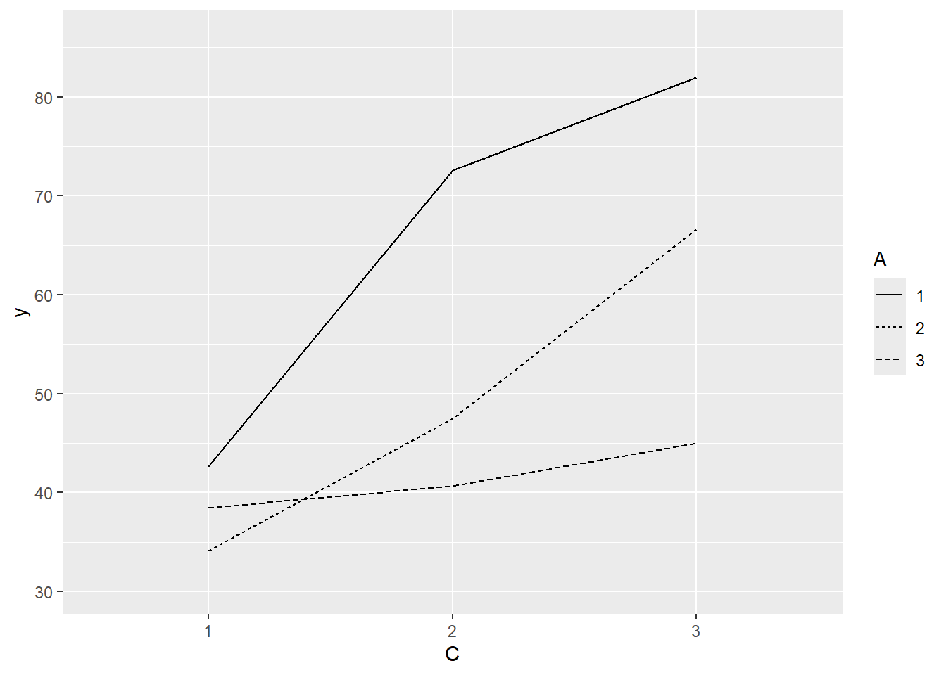
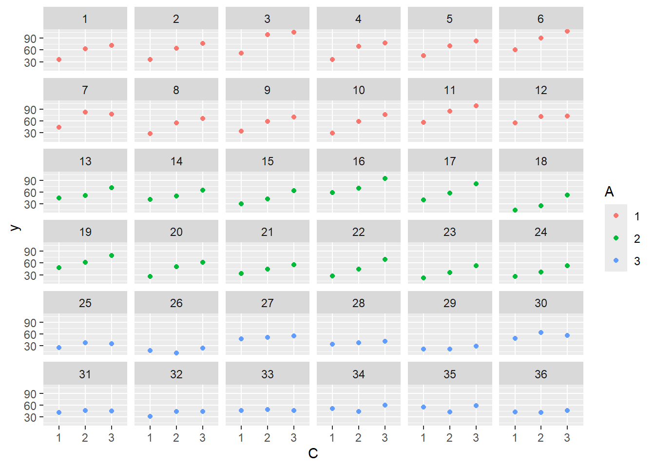
Imagine we has designed an experiment in which we intend to measure a response (\(y\)) to one of treatments (three levels; “a1”, “a2” and “a3”). Unfortunately, the system that we intend to sample is spatially heterogeneous and thus will add a great deal of noise to the data that will make it difficult to detect a signal (impact of treatment). Thus in an attempt to constrain this variability you decide to apply a design (RCB) in which each of the treatments within each of \(35\) blocks dispersed randomly throughout the landscape. As this section is mainly about the generation of artificial data (and not specifically about what to do with the data), understanding the actual details are optional and can be safely skipped.

library(plyr)
set.seed(123)
nA <- 3
nC <- 3
nBlock <- 36
sigma <- 5
sigma.block <- 12
n <- nBlock*nC
Block <- gl(nBlock, k=1)
C <- gl(nC,k=1)

## Specify the cell means
AC.means<-(rbind(c(40,70,80),c(35,50,70),c(35,40,45)))
## Convert these to effects
X <- model.matrix(~A*C,data=expand.grid(A=gl(3,k=1),C=gl(3,k=1)))
AC <- as.vector(AC.means)
AC.effects <- solve(X,AC)

A <- gl(nA,nBlock,n)
dt <- expand.grid(C=C,Block=Block)
dt <- data.frame(dt,A)

Xmat <- cbind(model.matrix(~-1+Block, data=dt),model.matrix(~A*C, data=dt))
block.effects <-  rnorm(n = nBlock, mean =0 , sd = sigma.block)
all.effects <- c(block.effects, AC.effects)
lin.pred <- Xmat %*% all.effects

## the quadrat observations (within sites) are drawn from
## normal distributions with means according to the site means
## and standard deviations of 5
y <- rnorm(n,lin.pred,sigma)
data.splt <- data.frame(y=y, A=A,dt)
head(data.splt)  #print out the first six rows of the data set

NA          y A C Block A.1
NA 1 36.04388 1 1     1   1
NA 2 62.96473 1 2     1   1
NA 3 71.74448 1 3     1   1
NA 4 35.33552 1 1     2   1
NA 5 63.76434 1 2     2   1
NA 6 76.19828 1 3     2   1

tapply(data.splt$y,data.splt$A,mean)

NA        1        2        3 
NA 65.71431 49.43047 41.36212

tapply(data.splt$y,data.splt$C,mean)

NA        1        2        3 
NA 38.41079 53.56792 64.52819

replications(y~A*C+Error(Block), data.splt)

NA   A   C A:C 
NA  36  36  12

library(ggplot2)
ggplot(data.splt, aes(y=y, x=C, linetype=A, group=A)) + geom_line(stat='summary', fun.y=mean)

ggplot(data.splt, aes(y=y, x=C,color=A)) + geom_point() + facet_wrap(~Block)

Exploratory data analysis

Normality and Homogeneity of variance

# check between plot effects
boxplot(y~A, ddply(data.splt,~A+Block, summarise,y=mean(y)))

#OR
ggplot(ddply(data.splt,~A+Block, summarise,y=mean(y)), aes(y=y, x=A)) + geom_boxplot()

# check within plot effects
boxplot(y~A*C, data.splt)

#OR 
ggplot(data.splt, aes(y=y, x=C, fill=A)) + geom_boxplot()

Conclusions:

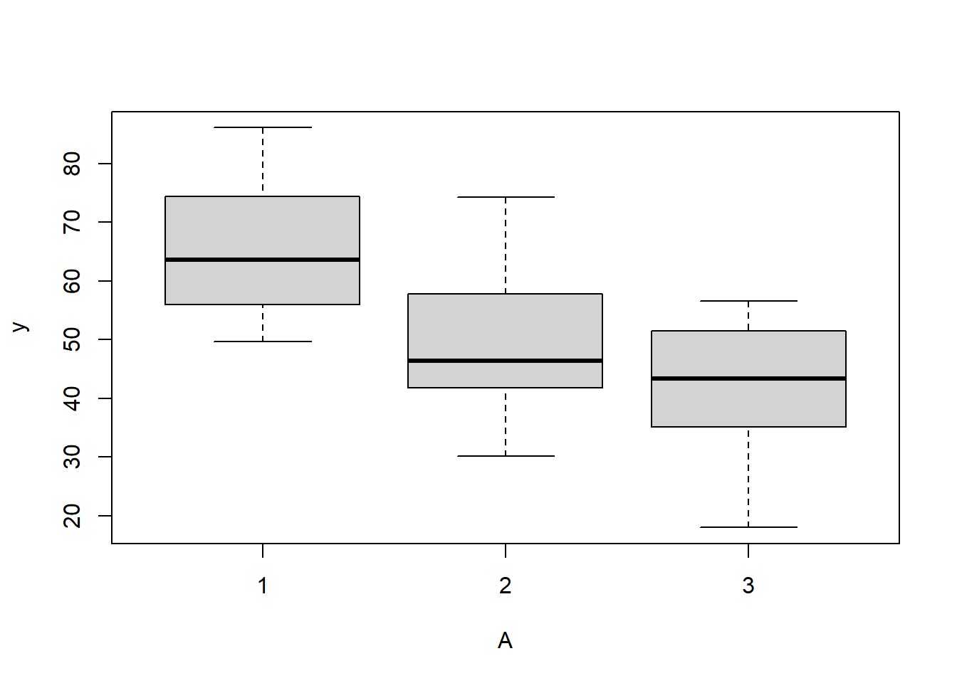
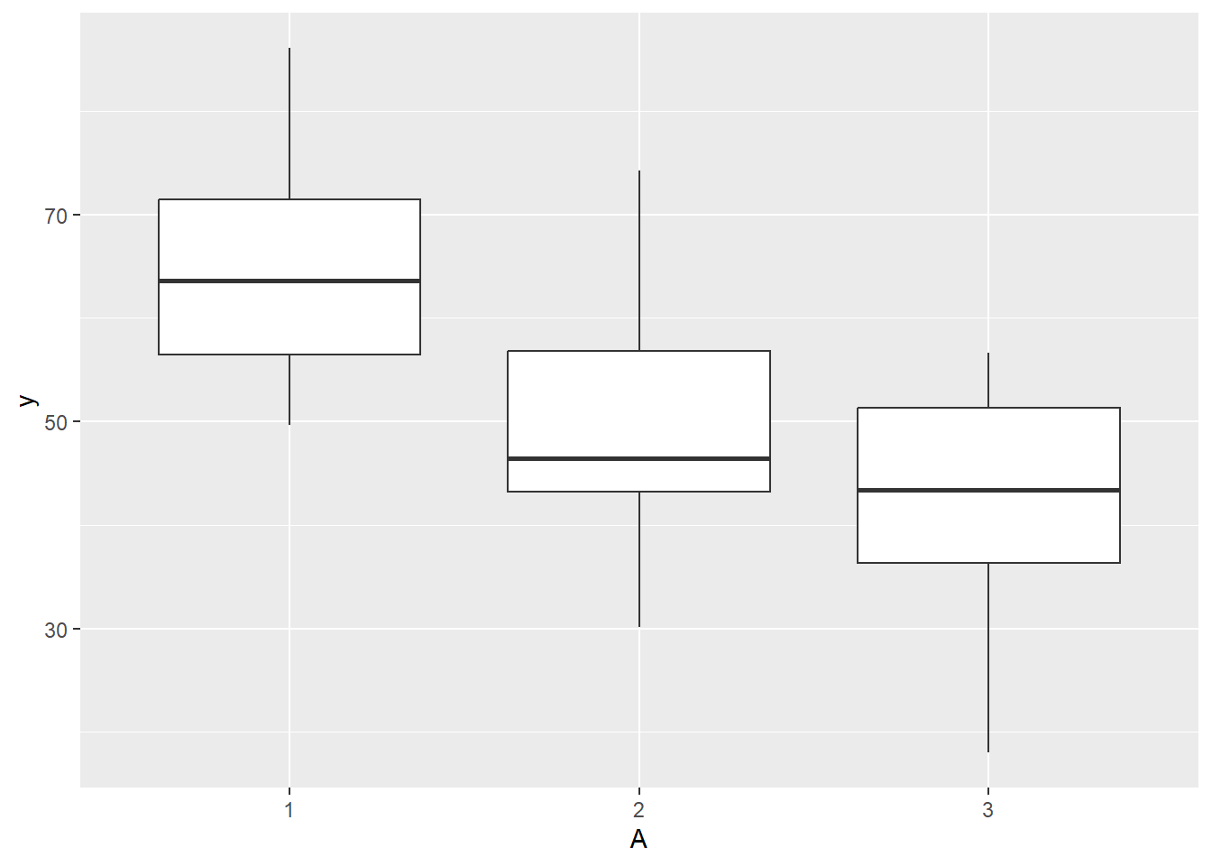
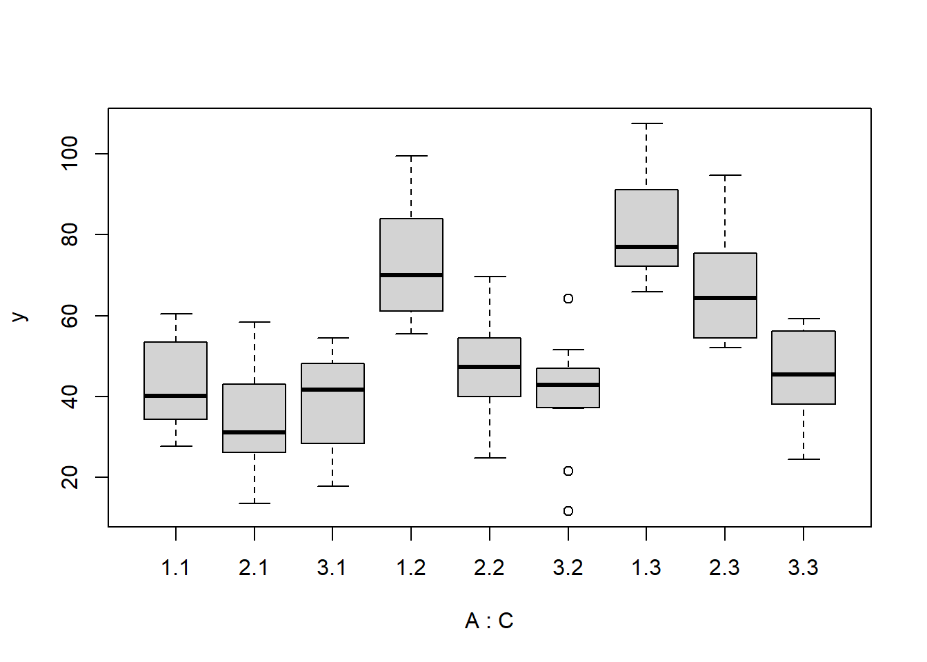
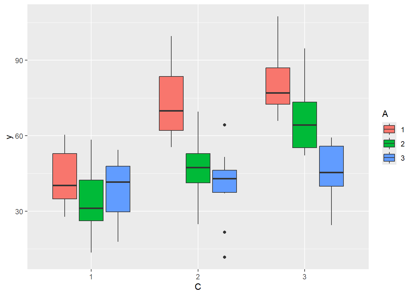
there is no evidence that the response variable is consistently non-normal across all populations - each boxplot is approximately symmetrical.
there is no evidence that variance (as estimated by the height of the boxplots) differs between the five populations. More importantly, there is no evidence of a relationship between mean and variance - the height of boxplots does not increase with increasing position along the y-axis. Hence it there is no evidence of non-homogeneity.

Obvious violations could be addressed either by:

transform the scale of the response variables (to address normality, etc). Note transformations should be applied to the entire response variable (not just those populations that are skewed).

Block by within-Block interaction

library(car)
with(data.splt, interaction.plot(C,Block,y))

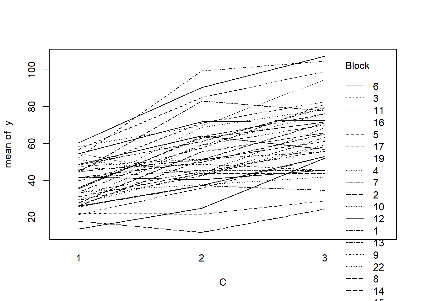
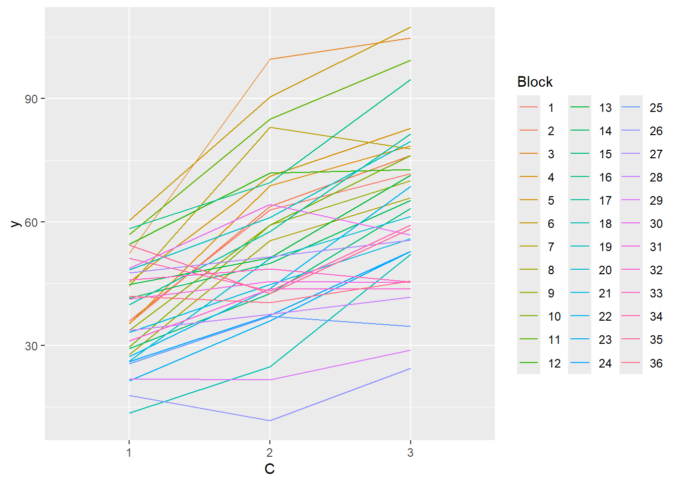
#OR with ggplot
library(ggplot2)
ggplot(data.splt, aes(y=y, x=C, group=Block,color=Block)) + geom_line() +
  guides(color=guide_legend(ncol=3))

residualPlots(lm(y~Block+A*C, data.splt))

NA            Test stat Pr(>|Test stat|)
NA Block                                
NA A                                    
NA C                                    
NA Tukey test    1.4518           0.1466

# the Tukey's non-additivity test by itself can be obtained via an internal function
# within the car package
car:::tukeyNonaddTest(lm(y~Block+A*C, data.splt))

NA      Test    Pvalue 
NA 1.4517644 0.1465671

Conclusions:

there is no visual or inferential evidence of any major interactions between Block and the within-Block effect (C). Any trends appear to be reasonably consistent between Blocks.

Example - split-plot

In an attempt to understand the effects on marine animals of short-term exposure to toxic substances, such as might occur following a spill, or a major increase in storm water flows, a it was decided to examine the toxicant in question, Copper, as part of a field experiment in Honk Kong. The experiment consisted of small sources of Cu (small, hemispherical plaster blocks, impregnated with copper), which released the metal into sea water over \(4\) or \(5\) days. The organism whose response to Cu was being measured was a small, polychaete worm, Hydroides, that attaches to hard surfaces in the sea, and is one of the first species to colonize any surface that is submerged. The biological questions focused on whether the timing of exposure to Cu affects the overall abundance of these worms. The time period of interest was the first or second week after a surface being available.

The experimental setup consisted of sheets of black perspex (settlement plates), which provided good surfaces for these worms. Each plate had a plaster block bolted to its centre, and the dissolving block would create a gradient of [Cu] across the plate. Over the two weeks of the experiment, a given plate would have pl ain plaster blocks (Control) or a block containing copper in the first week, followed by a plain block, or a plain block in the first week, followed by a dose of copper in the second week. After two weeks in the water, plates were removed and counted back in the laboratory. Without a clear idea of how sensitive these worms are to copper, an effect of the treatments might show up as an overall difference in the density of worms across a plate, or it could show up as a gradient in abundance across the plate, with a different gradient in different treatments. Therefore, on each plate, the density of worms was recorded at each of four distances from the center of the plate. Let’s have a look at the dataset

copper <- read.table('copper.csv', header=T, sep=',', strip.white=T)
head(copper)

NA    COPPER PLATE DIST WORMS
NA 1 control   200    4 11.50
NA 2 control   200    3 13.00
NA 3 control   200    2 13.50
NA 4 control   200    1 12.00
NA 5 control    39    4 17.75
NA 6 control    39    3 13.75

Variables’ description:

Copper. Categorical listing of the copper treatment (control = no copper applied, week 2 = copper treatment applied in second week and week 1= copper treatment applied in first week) applied to whole plates. Factor A (between plot factor).

Plate. Substrate provided for polychaete worm colonization on which copper treatment applied. These are the plots (Factor B). Numbers in this column represent numerical labels given to each plate.

Dist. Categorical listing for the four concentric distances from the center of the plate (source of copper treatment) with 1 being the closest and 4 the furthest. Factor C (within plot factor)

Worms. Density of worms measured. Response variable.

The Plates are the “random” groups. Within each Plate, all levels of the Distance factor occur (this is a within group factor). Each Plate can only be of one of the three levels of the Copper treatment. This is therefore a within group (nested) factor. Traditionally, this mixture of nested and randomised block design would be called a partly nested or split-plot design. In Bayesian (multilevel modeling) terms, this is a multi-level model with one hierarchical level the Plates means and another representing the Copper treatment means (based on the Plate means). Exploratory data analysis has indicated that the response variable could be normalised via a forth-root transformation.

Model fitting

We will only explore the matrix parameterisation (random intercepts) of the model, where

\[ \text{number of lesions}_i = \beta \text{Site}_{j(i)} + \epsilon_{i}, \]

where \(\epsilon_i∼ N(0,\sigma^2)\) and we treat Distance as a factor.

modelString="
model {
   #Likelihood
   for (i in 1:n) {
      y[i]~dnorm(mu[i],tau.res)
      mu[i] <- inprod(beta[],X[i,]) + inprod(gamma[],Z[i,])
      y.err[i] <- y[i] - mu[1]
   }

   #Priors and derivatives
   for (i in 1:nZ) {
      gamma[i] ~ dnorm(0,tau.plate)
   }
   for (i in 1:nX) {
      beta[i] ~ dnorm(0,1.0E-06)
   }

   tau.res <- pow(sigma.res,-2)
   sigma.res <- z/sqrt(chSq)
   z ~ dnorm(0, .0016)I(0,)
   chSq ~ dgamma(0.5, 0.5)

   tau.plate <- pow(sigma.plate,-2)
   sigma.plate <- z.plate/sqrt(chSq.plate)
   z.plate ~ dnorm(0, .0016)I(0,)
   chSq.plate ~ dgamma(0.5, 0.5)

 }
"

## write the model to a text file
writeLines(modelString, con = "matrixModel.txt")


#sort the data set so that the copper treatments are in a more logical order
library(dplyr)
copper$DIST <- factor(copper$DIST)
copper$PLATE <- factor(copper$PLATE)
copper.sort <- arrange(copper,COPPER,PLATE,DIST)

Xmat <- model.matrix(~COPPER*DIST, data=copper.sort)
Zmat <- model.matrix(~-1+PLATE, data=copper.sort)
copper.list <- list(y=copper.sort$WORMS,
               X=Xmat, nX=ncol(Xmat),
                           Z=Zmat, nZ=ncol(Zmat),
                           n=nrow(copper.sort)
                           )

params <- c("beta","gamma","sigma.res","sigma.plate")
burnInSteps = 1000
nChains = 2
numSavedSteps = 3000
thinSteps = 1
nIter = ceiling((numSavedSteps * thinSteps)/nChains)

library(R2jags)
library(coda)

copper.r2jags.b <- jags(data = copper.list, inits = NULL, parameters.to.save = params,
    model.file = "matrixModel.txt", n.chains = nChains, n.iter = nIter,
    n.burnin = burnInSteps, n.thin = thinSteps)

NA Compiling model graph
NA    Resolving undeclared variables
NA    Allocating nodes
NA Graph information:
NA    Observed stochastic nodes: 60
NA    Unobserved stochastic nodes: 31
NA    Total graph size: 1971
NA 
NA Initializing model

print(copper.r2jags.b)

NA Inference for Bugs model at "matrixModel.txt", fit using jags,
NA  2 chains, each with 1500 iterations (first 1000 discarded)
NA  n.sims = 1000 iterations saved
NA             mu.vect sd.vect    2.5%     25%     50%     75%   97.5%  Rhat n.eff
NA beta[1]      10.814   0.685   9.401  10.369  10.795  11.258  12.157 1.001  1000
NA beta[2]      -3.544   0.984  -5.440  -4.199  -3.525  -2.869  -1.574 1.002   640
NA beta[3]     -10.560   0.966 -12.615 -11.177 -10.559  -9.923  -8.712 1.003   610
NA beta[4]       1.172   0.884  -0.556   0.586   1.199   1.778   2.892 1.002  1000
NA beta[5]       1.582   0.878  -0.167   0.999   1.577   2.158   3.184 1.003  1000
NA beta[6]       2.743   0.857   1.039   2.151   2.719   3.342   4.443 1.003  1000
NA beta[7]      -0.073   1.233  -2.504  -0.875  -0.120   0.748   2.508 1.000  1000
NA beta[8]       0.007   1.271  -2.447  -0.792  -0.068   0.868   2.556 1.003  1000
NA beta[9]      -0.365   1.257  -2.866  -1.165  -0.397   0.499   1.960 1.000  1000
NA beta[10]      2.184   1.237  -0.254   1.395   2.183   2.954   4.846 1.007  1000
NA beta[11]     -0.008   1.204  -2.424  -0.763  -0.013   0.781   2.378 1.008   530
NA beta[12]      4.830   1.235   2.390   4.051   4.840   5.632   7.290 1.018  1000
NA gamma[1]      0.182   0.496  -0.719  -0.102   0.117   0.461   1.300 1.023   650
NA gamma[2]     -0.115   0.515  -1.218  -0.384  -0.074   0.153   0.915 1.020   300
NA gamma[3]      0.301   0.541  -0.720  -0.032   0.210   0.593   1.540 1.028   130
NA gamma[4]     -0.450   0.567  -1.733  -0.791  -0.359  -0.043   0.455 1.032    61
NA gamma[5]     -0.404   0.520  -1.489  -0.705  -0.328  -0.034   0.455 1.028   130
NA gamma[6]      0.867   0.712  -0.169   0.295   0.793   1.306   2.470 1.084    25
NA gamma[7]     -0.186   0.549  -1.386  -0.497  -0.120   0.106   0.856 1.011   290
NA gamma[8]     -0.530   0.589  -1.808  -0.936  -0.432  -0.051   0.326 1.059    35
NA gamma[9]      0.153   0.523  -0.919  -0.130   0.100   0.444   1.301 1.008  1000
NA gamma[10]    -0.154   0.512  -1.206  -0.452  -0.101   0.136   0.848 1.026   290
NA gamma[11]    -0.113   0.517  -1.317  -0.384  -0.078   0.181   0.896 1.004   920
NA gamma[12]     0.221   0.546  -0.780  -0.087   0.146   0.541   1.373 1.034   200
NA gamma[13]     0.136   0.520  -0.822  -0.170   0.081   0.400   1.345 1.017  1000
NA gamma[14]     0.171   0.541  -0.896  -0.123   0.106   0.466   1.345 1.019   470
NA gamma[15]    -0.085   0.500  -1.090  -0.374  -0.051   0.202   0.886 1.012  1000
NA sigma.plate   0.633   0.346   0.050   0.381   0.622   0.842   1.352 1.094    23
NA sigma.res     1.385   0.166   1.085   1.274   1.377   1.488   1.750 1.038    44
NA deviance    207.885   8.472 192.227 202.168 207.696 213.399 225.038 1.060    31
NA 
NA For each parameter, n.eff is a crude measure of effective sample size,
NA and Rhat is the potential scale reduction factor (at convergence, Rhat=1).
NA 
NA DIC info (using the rule, pD = var(deviance)/2)
NA pD = 34.7 and DIC = 242.6
NA DIC is an estimate of expected predictive error (lower deviance is better).

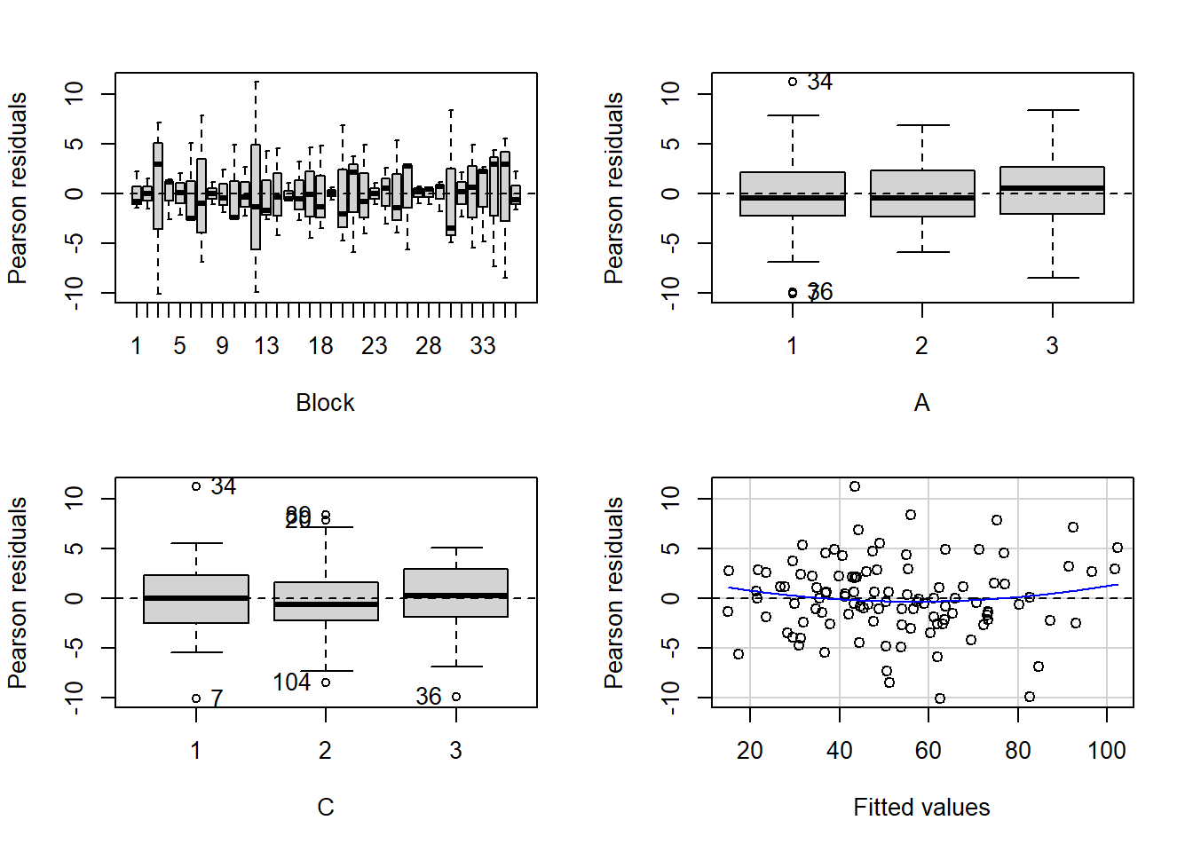
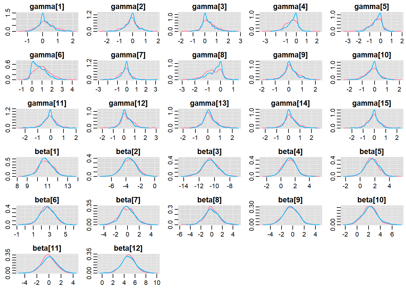
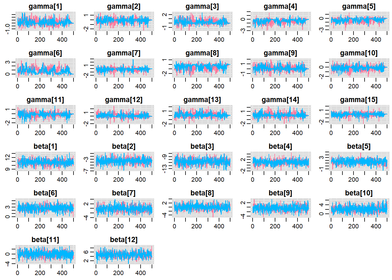
MCMC diagnostics

Before fully exploring the parameters, it is prudent to examine the convergence and mixing diagnostics. Chose either any of the parameterizations (they should yield much the same).

library(mcmcplots)
denplot(copper.r2jags.b, parms = c("gamma","beta"))

traplot(copper.r2jags.b, parms = c("gamma","beta"))

raftery.diag(as.mcmc(copper.r2jags.b))

NA [[1]]
NA 
NA Quantile (q) = 0.025
NA Accuracy (r) = +/- 0.005
NA Probability (s) = 0.95 
NA 
NA You need a sample size of at least 3746 with these values of q, r and s
NA 
NA [[2]]
NA 
NA Quantile (q) = 0.025
NA Accuracy (r) = +/- 0.005
NA Probability (s) = 0.95 
NA 
NA You need a sample size of at least 3746 with these values of q, r and s

autocorr.diag(as.mcmc(copper.r2jags.b))

NA             beta[1]     beta[2]      beta[3]      beta[4]      beta[5]
NA Lag 0   1.000000000  1.00000000  1.000000000  1.000000000  1.000000000
NA Lag 1   0.021272766  0.04648343  0.007883585 -0.031877909  0.005935939
NA Lag 5  -0.008158584 -0.04203414  0.003333370 -0.025041071 -0.049596493
NA Lag 10  0.031505586 -0.03660104  0.063264397  0.005126694  0.061062870
NA Lag 50 -0.027782043 -0.01419507 -0.063446191 -0.025966769  0.000139520
NA             beta[6]      beta[7]      beta[8]     beta[9]    beta[10]
NA Lag 0   1.000000000  1.000000000  1.000000000  1.00000000  1.00000000
NA Lag 1   0.003141284  0.006332145 -0.016090936  0.02230158 -0.01371002
NA Lag 5  -0.047609108 -0.015586534 -0.004392271 -0.04095146  0.03636817
NA Lag 10 -0.021534565  0.002483458  0.022938630  0.03931772  0.09976040
NA Lag 50  0.018649619  0.039287014 -0.026677246  0.02487322 -0.01257863
NA            beta[11]    beta[12]   deviance    gamma[1]    gamma[2]   gamma[3]
NA Lag 0   1.000000000  1.00000000 1.00000000  1.00000000  1.00000000 1.00000000
NA Lag 1   0.003598499  0.04451183 0.42158932  0.09957956  0.03142211 0.07683730
NA Lag 5  -0.048681325 -0.02569540 0.12353548  0.03983927 -0.00533499 0.02599357
NA Lag 10 -0.025741832 -0.01822980 0.08655390 -0.02625359  0.05903335 0.05050285
NA Lag 50  0.008573506 -0.02525275 0.02010397 -0.04670946 -0.04143951 0.01017881
NA           gamma[4]   gamma[5]   gamma[6]    gamma[7]    gamma[8]     gamma[9]
NA Lag 0   1.00000000 1.00000000  1.0000000  1.00000000  1.00000000  1.000000000
NA Lag 1   0.20659505 0.19599762  0.5113019  0.01034209  0.22908668  0.003942025
NA Lag 5   0.13726039 0.11488655  0.2890791 -0.07543631  0.15468366  0.039009815
NA Lag 10  0.08819534 0.06826430  0.1643047  0.03128544  0.03212642 -0.007477517
NA Lag 50 -0.03923514 0.01121642 -0.1002922 -0.01843480 -0.04706169 -0.012306197
NA           gamma[10]     gamma[11]    gamma[12]   gamma[13]   gamma[14]
NA Lag 0   1.000000000  1.0000000000  1.000000000  1.00000000 1.000000000
NA Lag 1   0.010206952  0.0028638893  0.009332531  0.03815594 0.007373479
NA Lag 5  -0.061360721  0.0008173756 -0.012857899 -0.02174086 0.022461865
NA Lag 10 -0.013288697 -0.0226321328  0.001324936  0.03479040 0.031318743
NA Lag 50  0.008887211 -0.0289618811 -0.026443165  0.01353287 0.037485638
NA           gamma[15] sigma.plate  sigma.res
NA Lag 0   1.000000000   1.0000000 1.00000000
NA Lag 1  -0.028327792   0.8371048 0.54229156
NA Lag 5  -0.010034686   0.5053673 0.03764157
NA Lag 10 -0.010388153   0.3404067 0.01350504
NA Lag 50  0.002533215  -0.1081944 0.07948304

Parameter estimates

print(copper.r2jags.b)

NA Inference for Bugs model at "matrixModel.txt", fit using jags,
NA  2 chains, each with 1500 iterations (first 1000 discarded)
NA  n.sims = 1000 iterations saved
NA             mu.vect sd.vect    2.5%     25%     50%     75%   97.5%  Rhat n.eff
NA beta[1]      10.814   0.685   9.401  10.369  10.795  11.258  12.157 1.001  1000
NA beta[2]      -3.544   0.984  -5.440  -4.199  -3.525  -2.869  -1.574 1.002   640
NA beta[3]     -10.560   0.966 -12.615 -11.177 -10.559  -9.923  -8.712 1.003   610
NA beta[4]       1.172   0.884  -0.556   0.586   1.199   1.778   2.892 1.002  1000
NA beta[5]       1.582   0.878  -0.167   0.999   1.577   2.158   3.184 1.003  1000
NA beta[6]       2.743   0.857   1.039   2.151   2.719   3.342   4.443 1.003  1000
NA beta[7]      -0.073   1.233  -2.504  -0.875  -0.120   0.748   2.508 1.000  1000
NA beta[8]       0.007   1.271  -2.447  -0.792  -0.068   0.868   2.556 1.003  1000
NA beta[9]      -0.365   1.257  -2.866  -1.165  -0.397   0.499   1.960 1.000  1000
NA beta[10]      2.184   1.237  -0.254   1.395   2.183   2.954   4.846 1.007  1000
NA beta[11]     -0.008   1.204  -2.424  -0.763  -0.013   0.781   2.378 1.008   530
NA beta[12]      4.830   1.235   2.390   4.051   4.840   5.632   7.290 1.018  1000
NA gamma[1]      0.182   0.496  -0.719  -0.102   0.117   0.461   1.300 1.023   650
NA gamma[2]     -0.115   0.515  -1.218  -0.384  -0.074   0.153   0.915 1.020   300
NA gamma[3]      0.301   0.541  -0.720  -0.032   0.210   0.593   1.540 1.028   130
NA gamma[4]     -0.450   0.567  -1.733  -0.791  -0.359  -0.043   0.455 1.032    61
NA gamma[5]     -0.404   0.520  -1.489  -0.705  -0.328  -0.034   0.455 1.028   130
NA gamma[6]      0.867   0.712  -0.169   0.295   0.793   1.306   2.470 1.084    25
NA gamma[7]     -0.186   0.549  -1.386  -0.497  -0.120   0.106   0.856 1.011   290
NA gamma[8]     -0.530   0.589  -1.808  -0.936  -0.432  -0.051   0.326 1.059    35
NA gamma[9]      0.153   0.523  -0.919  -0.130   0.100   0.444   1.301 1.008  1000
NA gamma[10]    -0.154   0.512  -1.206  -0.452  -0.101   0.136   0.848 1.026   290
NA gamma[11]    -0.113   0.517  -1.317  -0.384  -0.078   0.181   0.896 1.004   920
NA gamma[12]     0.221   0.546  -0.780  -0.087   0.146   0.541   1.373 1.034   200
NA gamma[13]     0.136   0.520  -0.822  -0.170   0.081   0.400   1.345 1.017  1000
NA gamma[14]     0.171   0.541  -0.896  -0.123   0.106   0.466   1.345 1.019   470
NA gamma[15]    -0.085   0.500  -1.090  -0.374  -0.051   0.202   0.886 1.012  1000
NA sigma.plate   0.633   0.346   0.050   0.381   0.622   0.842   1.352 1.094    23
NA sigma.res     1.385   0.166   1.085   1.274   1.377   1.488   1.750 1.038    44
NA deviance    207.885   8.472 192.227 202.168 207.696 213.399 225.038 1.060    31
NA 
NA For each parameter, n.eff is a crude measure of effective sample size,
NA and Rhat is the potential scale reduction factor (at convergence, Rhat=1).
NA 
NA DIC info (using the rule, pD = var(deviance)/2)
NA pD = 34.7 and DIC = 242.6
NA DIC is an estimate of expected predictive error (lower deviance is better).

References

Plummer, Martyn. 2004. “JAGS: Just Another Gibbs Sampler.”

Su, Yu-Sung, Masanao Yajima, Maintainer Yu-Sung Su, and JAGS SystemRequirements. 2015. “Package ‘R2jags’.” R Package Version 0.03-08, URL Http://CRAN. R-Project. Org/Package= R2jags.