This tutorial will focus on the use of Bayesian estimation to fit simple linear regression models …
Keywords
Software, Statistics, Stan
This tutorial will focus on the use of Bayesian estimation to fit simple linear regression models. BUGS (Bayesian inference Using Gibbs Sampling) is an algorithm and supporting language (resembling R) dedicated to performing the Gibbs sampling implementation of Markov Chain Monte Carlo (MCMC) method. Dialects of the BUGS language are implemented within three main projects:
OpenBUGS - written in component pascal.
JAGS - (Just Another Gibbs Sampler) - written in C++.
Stan - a dedicated Bayesian modelling framework written in C++ and implementing Hamiltonian MCMC samplers.
Whilst the above programs can be used stand-alone, they do offer the rich data pre-processing and graphical capabilities of R, and thus, they are best accessed from within R itself. As such there are multiple packages devoted to interfacing with the various software implementations:
R2OpenBUGS - interfaces with OpenBUGS
R2jags - interfaces with JAGS
rstan - interfaces with Stan
This tutorial will demonstrate how to fit models in Stan (Gelman, Lee, and Guo (2015)) using the package rstan (Stan Development Team (2018)) as interface, which also requires to load some other packages.
Overview
Introduction
In the previous tutorial (nested ANOVA), we introduced the concept of employing sub-replicates that are nested within the main treatment levels as a means of absorbing some of the unexplained variability that would otherwise arise from designs in which sampling units are selected from amongst highly heterogeneous conditions. Such (nested) designs are useful in circumstances where the levels of the main treatment (such as burnt and un-burnt sites) occur at a much larger temporal or spatial scale than the experimental/sampling units (e.g. vegetation monitoring quadrats). For circumstances in which the main treatments can be applied (or naturally occur) at the same scale as the sampling units (such as whether a stream rock is enclosed by a fish proof fence or not), an alternative design is available. In this design (randomised complete block design), each of the levels of the main treatment factor are grouped (blocked) together (in space and/or time) and therefore, whilst the conditions between the groups (referred to as “blocks”) might vary substantially, the conditions under which each of the levels of the treatment are tested within any given block are far more homogeneous.
If any differences between blocks (due to the heterogeneity) can account for some of the total variability between the sampling units (thereby reducing the amount of variability that the main treatment(s) failed to explain), then the main test of treatment effects will be more powerful/sensitive. As an simple example of a randomised complete block (RCB) design, consider an investigation into the roles of different organism scales (microbial, macro invertebrate and vertebrate) on the breakdown of leaf debris packs within streams. An experiment could consist of four treatment levels - leaf packs protected by fish-proof mesh, leaf packs protected by fine macro invertebrate exclusion mesh, leaf packs protected by dissolving antibacterial tablets, and leaf packs relatively unprotected as controls. As an acknowledgement that there are many other unmeasured factors that could influence leaf pack breakdown (such as flow velocity, light levels, etc) and that these are likely to vary substantially throughout a stream, the treatments are to be arranged into groups or “blocks” (each containing a single control, microbial, macro invertebrate and fish protected leaf pack). Blocks of treatment sets are then secured in locations haphazardly selected throughout a particular reach of stream. Importantly, the arrangement of treatments in each block must be randomized to prevent the introduction of some systematic bias - such as light angle, current direction etc.
Blocking does however come at a cost. The blocks absorb both unexplained variability as well as degrees of freedom from the residuals. Consequently, if the amount of the total unexplained variation that is absorbed by the blocks is not sufficiently large enough to offset the reduction in degrees of freedom (which may result from either less than expected heterogeneity, or due to the scale at which the blocks are established being inappropriate to explain much of the variation), for a given number of sampling units (leaf packs), the tests of main treatment effects will suffer power reductions. Treatments can also be applied sequentially or repeatedly at the scale of the entire block, such that at any single time, only a single treatment level is being applied (see the lower two sub-figures above). Such designs are called repeated measures. A repeated measures ANOVA is to an single factor ANOVA as a paired t-test is to a independent samples t-test. One example of a repeated measures analysis might be an investigation into the effects of a five different diet drugs (four doses and a placebo) on the food intake of lab rats. Each of the rats (“subjects”) is subject to each of the four drugs (within subject effects) which are administered in a random order. In another example, temporal recovery responses of sharks to bi-catch entanglement stresses might be simulated by analyzing blood samples collected from captive sharks (subjects) every half hour for three hours following a stress inducing restraint. This repeated measures design allows the anticipated variability in stress tolerances between individual sharks to be accounted for in the analysis (so as to permit more powerful test of the main treatments). Furthermore, by performing repeated measures on the same subjects, repeated measures designs reduce the number of subjects required for the investigation. Essentially, this is a randomised complete block design except that the within subject (block) effect (e.g. time since stress exposure) cannot be randomised.
To suppress contamination effects resulting from the proximity of treatment sampling units within a block, units should be adequately spaced in time and space. For example, the leaf packs should not be so close to one another that the control packs are effected by the antibacterial tablets and there should be sufficient recovery time between subsequent drug administrations. In addition, the order or arrangement of treatments within the blocks must be randomized so as to prevent both confounding as well as computational complications. Whilst this is relatively straight forward for the classic randomized complete block design (such as the leaf packs in streams), it is logically not possible for repeated measures designs. Blocking factors are typically random factors that represent all the possible blocks that could be selected. As such, no individual block can truly be replicated. Randomised complete block and repeated measures designs can therefore also be thought of as un-replicated factorial designs in which there are two or more factors but that the interactions between the blocks and all the within block factors are not replicated.
Linear models
The linear models for two and three factor nested design are:
where \(\mu\) is the overall mean, \(\beta\) is the effect of the Blocking Factor B (\(\sum \beta=0\)), \(\alpha\) and \(\gamma\) are the effects of withing block Factor A and Factor C, respectively, and \(\epsilon \sim N(0,\sigma^2)\) is the random unexplained or residual component.
Tests for the effects of blocks as well as effects within blocks assume that there are no interactions between blocks and the within block effects. That is, it is assumed that any effects are of similar nature within each of the blocks. Whilst this assumption may well hold for experiments that are able to consciously set the scale over which the blocking units are arranged, when designs utilize arbitrary or naturally occurring blocking units, the magnitude and even polarity of the main effects are likely to vary substantially between the blocks. The preferred (non-additive or “Model 1”) approach to un-replicated factorial analysis of some bio-statisticians is to include the block by within subject effect interactions (e.g. \(\beta\alpha\)). Whilst these interaction effects cannot be formally tested, they can be used as the denominators in F-ratio calculations of their respective main effects tests. Proponents argue that since these blocking interactions cannot be formally tested, there is no sound inferential basis for using these error terms separately. Alternatively, models can be fitted additively (“Model 2”) whereby all the block by within subject effect interactions are pooled into a single residual term (\(\epsilon\)). Although the latter approach is simpler, each of the within subject effects tests do assume that there are no interactions involving the blocks and that perhaps even more restrictively, that sphericity holds across the entire design.
Assumptions
As with other ANOVA designs, the reliability of hypothesis tests is dependent on the residuals being:
normally distributed. Boxplots using the appropriate scale of replication (reflecting the appropriate residuals/F-ratio denominator should be used to explore normality. Scale transformations are often useful.
equally varied. Boxplots and plots of means against variance (using the appropriate scale of replication) should be used to explore the spread of values. Residual plots should reveal no patterns. Scale transformations are often useful.
independent of one another. Although the observations within a block may not strictly be independent, provided the treatments are applied or ordered randomly within each block or subject, within block proximity effects on the residuals should be random across all blocks and thus the residuals should still be independent of one another. Nevertheless, it is important that experimental units within blocks are adequately spaced in space and time so as to suppress contamination or carryover effects.
Simple RCB
Data generation
Imagine we has designed an experiment in which we intend to measure a response (y) to one of treatments (three levels; “a1”, “a2” and “a3”). Unfortunately, the system that we intend to sample is spatially heterogeneous and thus will add a great deal of noise to the data that will make it difficult to detect a signal (impact of treatment). Thus in an attempt to constrain this variability you decide to apply a design (RCB) in which each of the treatments within each of 35 blocks dispersed randomly throughout the landscape. As this section is mainly about the generation of artificial data (and not specifically about what to do with the data), understanding the actual details are optional and can be safely skipped.
library(plyr)set.seed(123)nTreat <-3nBlock <-35sigma <-5sigma.block <-12n <- nBlock*nTreatBlock <-gl(nBlock, k=1)A <-gl(nTreat,k=1)dt <-expand.grid(A=A,Block=Block)#Xmat <- model.matrix(~Block + A + Block:A, data=dt)Xmat <-model.matrix(~-1+Block + A, data=dt)block.effects <-rnorm(n = nBlock, mean =40, sd = sigma.block)A.effects <-c(30,40)all.effects <-c(block.effects,A.effects)lin.pred <- Xmat %*% all.effects# ORXmat <-cbind(model.matrix(~-1+Block,data=dt),model.matrix(~-1+A,data=dt))## Sum to zero block effectsblock.effects <-rnorm(n = nBlock, mean =0, sd = sigma.block)A.effects <-c(40,70,80)all.effects <-c(block.effects,A.effects)lin.pred <- Xmat %*% all.effects## the quadrat observations (within sites) are drawn from## normal distributions with means according to the site means## and standard deviations of 5y <-rnorm(n,lin.pred,sigma)data.rcb <-data.frame(y=y, expand.grid(A=A, Block=Block))head(data.rcb) #print out the first six rows of the data set
NA          y A Block
NA 1 45.80853 1     1
NA 2 66.71784 2     1
NA 3 93.29238 3     1
NA 4 43.10101 1     2
NA 5 73.20697 2     2
NA 6 91.77487 3     2
Exploratory data analysis
Normality and Homogeneity of variance
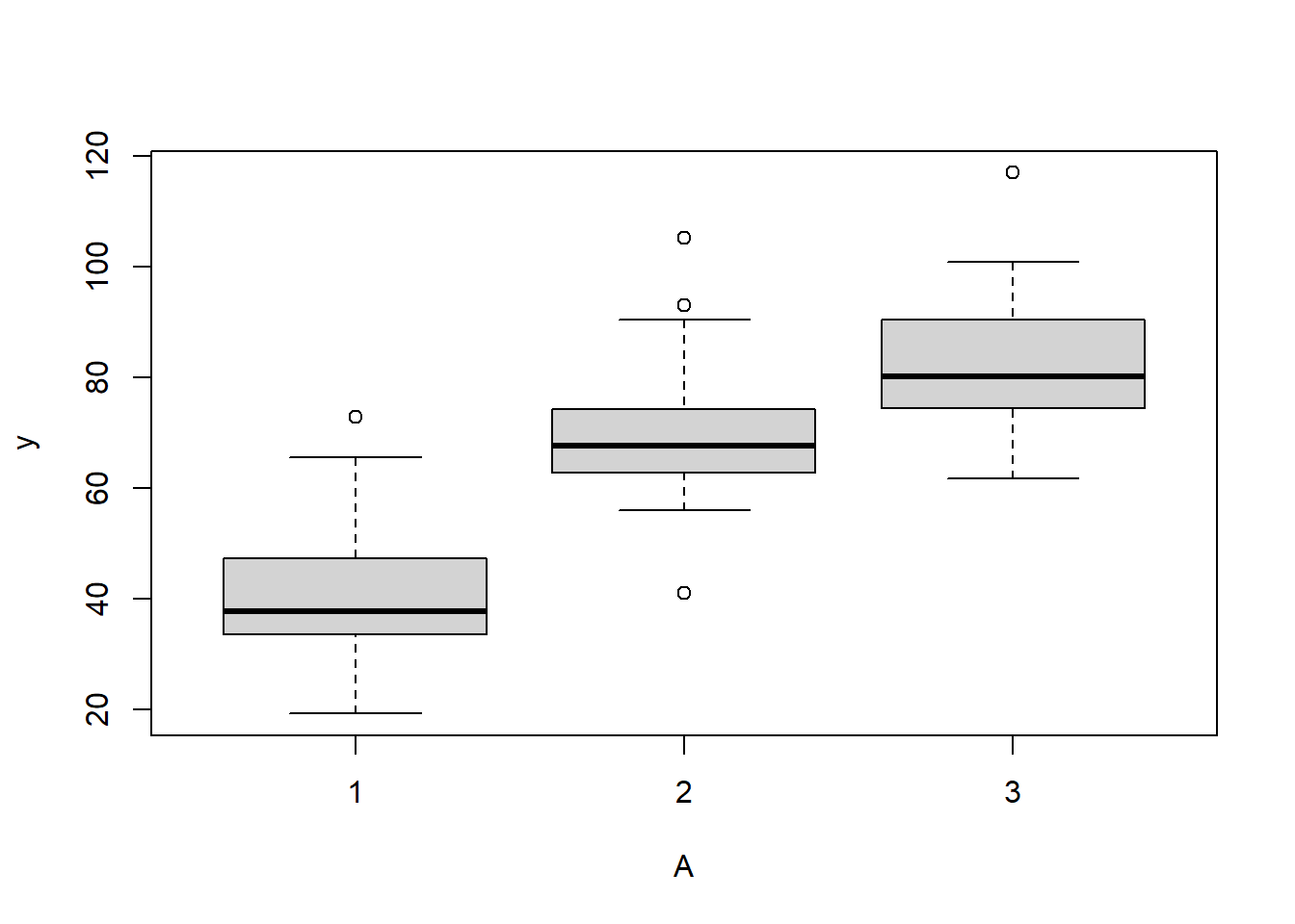
boxplot(y~A, data.rcb)
Conclusions:
there is no evidence that the response variable is consistently non-normal across all populations - each boxplot is approximately symmetrical.
there is no evidence that variance (as estimated by the height of the boxplots) differs between the five populations. . More importantly, there is no evidence of a relationship between mean and variance - the height of boxplots does not increase with increasing position along the \(y\)-axis. Hence it there is no evidence of non-homogeneity
Obvious violations could be addressed either by:
transform the scale of the response variables (to address normality, etc). Note transformations should be applied to the entire response variable (not just those populations that are skewed).
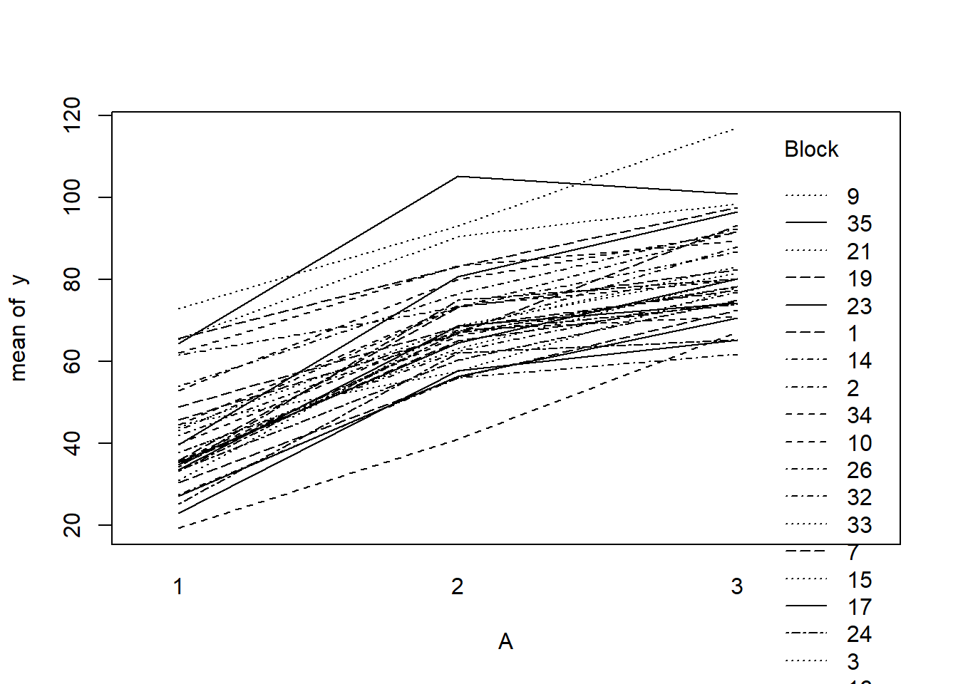
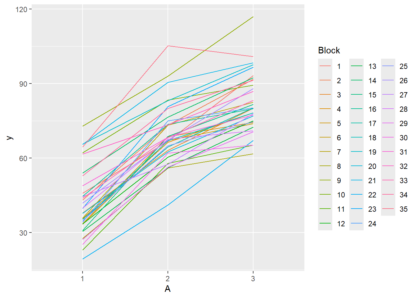
Block by within-Block interaction
library(car)with(data.rcb, interaction.plot(A,Block,y))#OR with ggplotlibrary(ggplot2)
NA            Test stat Pr(>|Test stat|)
NA Block
NA A
NA Tukey test   -1.4163           0.1567
# the Tukey's non-additivity test by itself can be obtained via an internal function# within the car packagecar:::tukeyNonaddTest(lm(y~Block+A, data.rcb))
NA       Test     Pvalue
NA -1.4163343  0.1566776
# alternatively, there is also a Tukey's non-additivity test within the# asbio packagelibrary(asbio)with(data.rcb,tukey.add.test(y,A,Block))
NA
NA Tukey's one df test for additivity
NA F = 2.0060029   Denom df = 67    p-value = 0.1613102
Conclusions:
there is no visual or inferential evidence of any major interactions between Block and the within-Block effect (A). Any trends appear to be reasonably consistent between Blocks.
where \(\gamma_{ij)} \sim N(0, \sigma^2_B)\), \(\beta_0, \beta_i \sim N(0, 1000000)\), and \(\sigma^2, \sigma^2_B \sim \text{Cauchy(0, 25)}\). The full parameterisation, shows the effects parameterisation in which there is an intercept (\(\beta_0\)) and two treatment effects (\(\beta_i\), where \(i\) is \(1,2\)).
where \(\gamma_{ij} \sim N(0, \sigma^2_B)\), \(\boldsymbol \beta \sim MVN(0, 1000000)\), and \(\sigma^2, \sigma^2_B \sim \text{Cauchy(0, 25)}\). The full parameterisation, shows the effects parameterisation in which there is an intercept (\(\alpha_0\)) and two treatment effects (\(\beta_i\), where \(i\) is \(1,2\)). The matrix parameterisation is a compressed notation, In this parameterisation, there are three alpha parameters (one representing the mean of treatment a1, and the other two representing the treatment effects (differences between a2 and a1 and a3 and a1). In generating priors for each of these three alpha parameters, we could loop through each and define a non-informative normal prior to each (as in the Full parameterisation version). However, it turns out that it is more efficient (in terms of mixing and thus the number of necessary iterations) to define the priors from a multivariate normal distribution. This has as many means as there are parameters to estimate (\(3\)) and a \(3\times3\) matrix of zeros and \(100\) in the diagonals.
where \(\gamma_{ij} \sim N(0, \sigma^2_B)\), \(\beta_0, \beta_i \sim N(0, 1000000)\), and \(\sigma^2, \sigma^2_B \sim \text{Cauchy(0, 25)}\).
Rather than assume a specific variance-covariance structure, just like lme we can incorporate an appropriate structure to account for different dependency/correlation structures in our data. In RCB designs, it is prudent to capture the residuals to allow checks that there are no outstanding dependency issues following model fitting.
Full means parameterisation
rstanString="data{ int n; int nA; int nB; vector [n] y; int A[n]; int B[n];}parameters{ real alpha[nA]; real<lower=0> sigma; vector [nB] beta; real<lower=0> sigma_B;}model{ real mu[n]; // Priors alpha ~ normal( 0 , 100 ); beta ~ normal( 0 , sigma_B ); sigma_B ~ cauchy( 0 , 25 ); sigma ~ cauchy( 0 , 25 ); for ( i in 1:n ) { mu[i] = alpha[A[i]] + beta[B[i]]; } y ~ normal( mu , sigma );}"## write the model to a text filewriteLines(rstanString, con ="fullModel.stan")
Arrange the data as a list (as required by Stan). As input, Stan will need to be supplied with: the response variable, the predictor matrix, the number of predictors, the total number of observed items. This all needs to be contained within a list object. We will create two data lists, one for each of the hypotheses.
NA
NA SAMPLING FOR MODEL 'anon_model' NOW (CHAIN 1).
NA Chain 1:
NA Chain 1: Gradient evaluation took 3.7e-05 seconds
NA Chain 1: 1000 transitions using 10 leapfrog steps per transition would take 0.37 seconds.
NA Chain 1: Adjust your expectations accordingly!
NA Chain 1:
NA Chain 1:
NA Chain 1: Iteration:    1 / 4500 [  0%]  (Warmup)
NA Chain 1: Iteration:  450 / 4500 [ 10%]  (Warmup)
NA Chain 1: Iteration:  900 / 4500 [ 20%]  (Warmup)
NA Chain 1: Iteration: 1350 / 4500 [ 30%]  (Warmup)
NA Chain 1: Iteration: 1800 / 4500 [ 40%]  (Warmup)
NA Chain 1: Iteration: 2250 / 4500 [ 50%]  (Warmup)
NA Chain 1: Iteration: 2700 / 4500 [ 60%]  (Warmup)
NA Chain 1: Iteration: 3001 / 4500 [ 66%]  (Sampling)
NA Chain 1: Iteration: 3450 / 4500 [ 76%]  (Sampling)
NA Chain 1: Iteration: 3900 / 4500 [ 86%]  (Sampling)
NA Chain 1: Iteration: 4350 / 4500 [ 96%]  (Sampling)
NA Chain 1: Iteration: 4500 / 4500 [100%]  (Sampling)
NA Chain 1:
NA Chain 1:  Elapsed Time: 0.243 seconds (Warm-up)
NA Chain 1:                0.111 seconds (Sampling)
NA Chain 1:                0.354 seconds (Total)
NA Chain 1:
NA
NA SAMPLING FOR MODEL 'anon_model' NOW (CHAIN 2).
NA Chain 2:
NA Chain 2: Gradient evaluation took 7e-06 seconds
NA Chain 2: 1000 transitions using 10 leapfrog steps per transition would take 0.07 seconds.
NA Chain 2: Adjust your expectations accordingly!
NA Chain 2:
NA Chain 2:
NA Chain 2: Iteration:    1 / 4500 [  0%]  (Warmup)
NA Chain 2: Iteration:  450 / 4500 [ 10%]  (Warmup)
NA Chain 2: Iteration:  900 / 4500 [ 20%]  (Warmup)
NA Chain 2: Iteration: 1350 / 4500 [ 30%]  (Warmup)
NA Chain 2: Iteration: 1800 / 4500 [ 40%]  (Warmup)
NA Chain 2: Iteration: 2250 / 4500 [ 50%]  (Warmup)
NA Chain 2: Iteration: 2700 / 4500 [ 60%]  (Warmup)
NA Chain 2: Iteration: 3001 / 4500 [ 66%]  (Sampling)
NA Chain 2: Iteration: 3450 / 4500 [ 76%]  (Sampling)
NA Chain 2: Iteration: 3900 / 4500 [ 86%]  (Sampling)
NA Chain 2: Iteration: 4350 / 4500 [ 96%]  (Sampling)
NA Chain 2: Iteration: 4500 / 4500 [100%]  (Sampling)
NA Chain 2:
NA Chain 2:  Elapsed Time: 0.237 seconds (Warm-up)
NA Chain 2:                0.105 seconds (Sampling)
NA Chain 2:                0.342 seconds (Total)
NA Chain 2:
print(data.rcb.rstan.c, par =c("alpha", "sigma", "sigma_B"))
NA Inference for Stan model: anon_model.
NA 2 chains, each with iter=4500; warmup=3000; thin=1;
NA post-warmup draws per chain=1500, total post-warmup draws=3000.
NA
NA           mean se_mean   sd  2.5%   25%   50%   75% 97.5% n_eff Rhat
NA alpha[1] 41.55    0.10 2.13 37.40 40.15 41.54 42.94 45.68   441 1.01
NA alpha[2] 69.50    0.11 2.16 65.31 68.08 69.50 70.86 73.85   419 1.01
NA alpha[3] 81.85    0.10 2.12 77.71 80.45 81.80 83.21 85.95   425 1.01
NA sigma     5.07    0.01 0.44  4.29  4.75  5.05  5.35  6.00  2176 1.00
NA sigma_B  11.71    0.03 1.60  9.10 10.58 11.55 12.63 15.35  3757 1.00
NA
NA Samples were drawn using NUTS(diag_e) at Mon Jul 22 12:08:01 2024.
NA For each parameter, n_eff is a crude measure of effective sample size,
NA and Rhat is the potential scale reduction factor on split chains (at
NA convergence, Rhat=1).
NA        X1      Median         X0.        X25.        X50.        X75.
NA 1 alpha.1   41.535980   32.655709   40.149101   41.535980   42.944616
NA 2 alpha.2   69.496977   61.677410   68.079227   69.496977   70.861836
NA 3 alpha.3   81.799857   73.717659   80.452339   81.799857   83.205086
NA 4   sigma    5.048656    3.677651    4.748179    5.048656    5.349604
NA 5 sigma_B   11.554897    7.586198   10.576991   11.554897   12.629219
NA 6    lp__ -321.666229 -342.185020 -325.626894 -321.666229 -318.292350
NA         X100.       lower       upper     lower.1    upper.1
NA 1   50.527411   37.476978   45.726479   40.282467   43.04881
NA 2   78.798149   65.297631   73.829659   68.437537   71.17360
NA 3   90.863749   77.678551   85.948313   80.381917   83.10695
NA 4    6.931274    4.212814    5.902948    4.673778    5.25575
NA 5   19.103937    8.800251   14.887844   10.404933   12.39880
NA 6 -307.824839 -333.210469 -312.359491 -325.688234 -318.38516
Full effect parameterisation
rstan2String="data{ int n; int nB; vector [n] y; int A2[n]; int A3[n]; int B[n];}parameters{ real alpha0; real alpha2; real alpha3; real<lower=0> sigma; vector [nB] beta; real<lower=0> sigma_B;}model{ real mu[n]; // Priors alpha0 ~ normal( 0 , 1000 ); alpha2 ~ normal( 0 , 1000 ); alpha3 ~ normal( 0 , 1000 ); beta ~ normal( 0 , sigma_B ); sigma_B ~ cauchy( 0 , 25 ); sigma ~ cauchy( 0 , 25 ); for ( i in 1:n ) { mu[i] = alpha0 + alpha2*A2[i] + alpha3*A3[i] + beta[B[i]]; } y ~ normal( mu , sigma );}"## write the model to a text filewriteLines(rstan2String, con ="full2Model.stan")
Arrange the data as a list (as required by Stan). As input, Stan will need to be supplied with: the response variable, the predictor matrix, the number of predictors, the total number of observed items. This all needs to be contained within a list object. We will create two data lists, one for each of the hypotheses.
NA
NA SAMPLING FOR MODEL 'anon_model' NOW (CHAIN 1).
NA Chain 1:
NA Chain 1: Gradient evaluation took 3.2e-05 seconds
NA Chain 1: 1000 transitions using 10 leapfrog steps per transition would take 0.32 seconds.
NA Chain 1: Adjust your expectations accordingly!
NA Chain 1:
NA Chain 1:
NA Chain 1: Iteration:    1 / 4500 [  0%]  (Warmup)
NA Chain 1: Iteration:  450 / 4500 [ 10%]  (Warmup)
NA Chain 1: Iteration:  900 / 4500 [ 20%]  (Warmup)
NA Chain 1: Iteration: 1350 / 4500 [ 30%]  (Warmup)
NA Chain 1: Iteration: 1800 / 4500 [ 40%]  (Warmup)
NA Chain 1: Iteration: 2250 / 4500 [ 50%]  (Warmup)
NA Chain 1: Iteration: 2700 / 4500 [ 60%]  (Warmup)
NA Chain 1: Iteration: 3001 / 4500 [ 66%]  (Sampling)
NA Chain 1: Iteration: 3450 / 4500 [ 76%]  (Sampling)
NA Chain 1: Iteration: 3900 / 4500 [ 86%]  (Sampling)
NA Chain 1: Iteration: 4350 / 4500 [ 96%]  (Sampling)
NA Chain 1: Iteration: 4500 / 4500 [100%]  (Sampling)
NA Chain 1:
NA Chain 1:  Elapsed Time: 0.421 seconds (Warm-up)
NA Chain 1:                0.165 seconds (Sampling)
NA Chain 1:                0.586 seconds (Total)
NA Chain 1:
NA
NA SAMPLING FOR MODEL 'anon_model' NOW (CHAIN 2).
NA Chain 2:
NA Chain 2: Gradient evaluation took 8e-06 seconds
NA Chain 2: 1000 transitions using 10 leapfrog steps per transition would take 0.08 seconds.
NA Chain 2: Adjust your expectations accordingly!
NA Chain 2:
NA Chain 2:
NA Chain 2: Iteration:    1 / 4500 [  0%]  (Warmup)
NA Chain 2: Iteration:  450 / 4500 [ 10%]  (Warmup)
NA Chain 2: Iteration:  900 / 4500 [ 20%]  (Warmup)
NA Chain 2: Iteration: 1350 / 4500 [ 30%]  (Warmup)
NA Chain 2: Iteration: 1800 / 4500 [ 40%]  (Warmup)
NA Chain 2: Iteration: 2250 / 4500 [ 50%]  (Warmup)
NA Chain 2: Iteration: 2700 / 4500 [ 60%]  (Warmup)
NA Chain 2: Iteration: 3001 / 4500 [ 66%]  (Sampling)
NA Chain 2: Iteration: 3450 / 4500 [ 76%]  (Sampling)
NA Chain 2: Iteration: 3900 / 4500 [ 86%]  (Sampling)
NA Chain 2: Iteration: 4350 / 4500 [ 96%]  (Sampling)
NA Chain 2: Iteration: 4500 / 4500 [100%]  (Sampling)
NA Chain 2:
NA Chain 2:  Elapsed Time: 0.445 seconds (Warm-up)
NA Chain 2:                0.175 seconds (Sampling)
NA Chain 2:                0.62 seconds (Total)
NA Chain 2:
print(data.rcb.rstan.f, par =c("alpha0", "alpha2", "alpha3", "sigma", "sigma_B"))
NA Inference for Stan model: anon_model.
NA 2 chains, each with iter=4500; warmup=3000; thin=1;
NA post-warmup draws per chain=1500, total post-warmup draws=3000.
NA
NA          mean se_mean   sd  2.5%   25%   50%   75% 97.5% n_eff Rhat
NA alpha0  41.73    0.14 2.17 37.48 40.25 41.70 43.24 46.17   253    1
NA alpha2  27.91    0.03 1.23 25.49 27.10 27.93 28.70 30.30  1991    1
NA alpha3  40.24    0.03 1.19 37.85 39.44 40.26 41.04 42.52  2033    1
NA sigma    5.08    0.01 0.46  4.28  4.76  5.05  5.37  6.07  1685    1
NA sigma_B 11.73    0.03 1.57  9.15 10.63 11.57 12.63 15.27  2206    1
NA
NA Samples were drawn using NUTS(diag_e) at Mon Jul 22 12:08:33 2024.
NA For each parameter, n_eff is a crude measure of effective sample size,
NA and Rhat is the potential scale reduction factor on split chains (at
NA convergence, Rhat=1).
NA        X1      Median         X0.        X25.        X50.        X75.
NA 1  alpha0   41.698390   34.473108   40.246925   41.698390   43.235888
NA 2  alpha2   27.929974   23.249223   27.096648   27.929974   28.701302
NA 3  alpha3   40.264280   35.080170   39.437859   40.264280   41.043282
NA 4   sigma    5.052888    3.786100    4.757611    5.052888    5.366813
NA 5 sigma_B   11.567793    7.661363   10.634201   11.567793   12.631537
NA 6    lp__ -321.145807 -342.911147 -325.003745 -321.145807 -317.615781
NA         X100.       lower       upper     lower.1     upper.1
NA 1   48.769516   37.757085   46.360518   40.444880   43.392733
NA 2   32.665468   25.650646   30.418299   27.152255   28.743241
NA 3   44.938585   37.833235   42.486534   39.485525   41.085516
NA 4    7.054157    4.214457    5.954861    4.688346    5.269776
NA 5   19.027742    9.063056   15.130256   10.347573   12.291484
NA 6 -306.630367 -332.364491 -310.979729 -323.592133 -316.356397
Matrix parameterisation
rstanString2="data{ int n; int nX; int nB; vector [n] y; matrix [n,nX] X; int B[n];}parameters{ vector [nX] beta; real<lower=0> sigma; vector [nB] gamma; real<lower=0> sigma_B;}transformed parameters { vector[n] mu; mu = X*beta; for (i in 1:n) { mu[i] = mu[i] + gamma[B[i]]; }} model{ // Priors beta ~ normal( 0 , 100 ); gamma ~ normal( 0 , sigma_B ); sigma_B ~ cauchy( 0 , 25 ); sigma ~ cauchy( 0 , 25 ); y ~ normal( mu , sigma );}"## write the model to a text filewriteLines(rstanString2, con ="matrixModel.stan")
Arrange the data as a list (as required by Stan). As input, Stan will need to be supplied with: the response variable, the predictor matrix, the number of predictors, the total number of observed items. This all needs to be contained within a list object. We will create two data lists, one for each of the hypotheses.
NA
NA SAMPLING FOR MODEL 'anon_model' NOW (CHAIN 1).
NA Chain 1:
NA Chain 1: Gradient evaluation took 3.9e-05 seconds
NA Chain 1: 1000 transitions using 10 leapfrog steps per transition would take 0.39 seconds.
NA Chain 1: Adjust your expectations accordingly!
NA Chain 1:
NA Chain 1:
NA Chain 1: Iteration:    1 / 4500 [  0%]  (Warmup)
NA Chain 1: Iteration:  450 / 4500 [ 10%]  (Warmup)
NA Chain 1: Iteration:  900 / 4500 [ 20%]  (Warmup)
NA Chain 1: Iteration: 1350 / 4500 [ 30%]  (Warmup)
NA Chain 1: Iteration: 1800 / 4500 [ 40%]  (Warmup)
NA Chain 1: Iteration: 2250 / 4500 [ 50%]  (Warmup)
NA Chain 1: Iteration: 2700 / 4500 [ 60%]  (Warmup)
NA Chain 1: Iteration: 3001 / 4500 [ 66%]  (Sampling)
NA Chain 1: Iteration: 3450 / 4500 [ 76%]  (Sampling)
NA Chain 1: Iteration: 3900 / 4500 [ 86%]  (Sampling)
NA Chain 1: Iteration: 4350 / 4500 [ 96%]  (Sampling)
NA Chain 1: Iteration: 4500 / 4500 [100%]  (Sampling)
NA Chain 1:
NA Chain 1:  Elapsed Time: 0.343 seconds (Warm-up)
NA Chain 1:                0.128 seconds (Sampling)
NA Chain 1:                0.471 seconds (Total)
NA Chain 1:
NA
NA SAMPLING FOR MODEL 'anon_model' NOW (CHAIN 2).
NA Chain 2:
NA Chain 2: Gradient evaluation took 8e-06 seconds
NA Chain 2: 1000 transitions using 10 leapfrog steps per transition would take 0.08 seconds.
NA Chain 2: Adjust your expectations accordingly!
NA Chain 2:
NA Chain 2:
NA Chain 2: Iteration:    1 / 4500 [  0%]  (Warmup)
NA Chain 2: Iteration:  450 / 4500 [ 10%]  (Warmup)
NA Chain 2: Iteration:  900 / 4500 [ 20%]  (Warmup)
NA Chain 2: Iteration: 1350 / 4500 [ 30%]  (Warmup)
NA Chain 2: Iteration: 1800 / 4500 [ 40%]  (Warmup)
NA Chain 2: Iteration: 2250 / 4500 [ 50%]  (Warmup)
NA Chain 2: Iteration: 2700 / 4500 [ 60%]  (Warmup)
NA Chain 2: Iteration: 3001 / 4500 [ 66%]  (Sampling)
NA Chain 2: Iteration: 3450 / 4500 [ 76%]  (Sampling)
NA Chain 2: Iteration: 3900 / 4500 [ 86%]  (Sampling)
NA Chain 2: Iteration: 4350 / 4500 [ 96%]  (Sampling)
NA Chain 2: Iteration: 4500 / 4500 [100%]  (Sampling)
NA Chain 2:
NA Chain 2:  Elapsed Time: 0.338 seconds (Warm-up)
NA Chain 2:                0.127 seconds (Sampling)
NA Chain 2:                0.465 seconds (Total)
NA Chain 2:
print(data.rcb.rstan.d, par =c("beta", "sigma", "sigma_B"))
NA Inference for Stan model: anon_model.
NA 2 chains, each with iter=4500; warmup=3000; thin=1;
NA post-warmup draws per chain=1500, total post-warmup draws=3000.
NA
NA          mean se_mean   sd  2.5%   25%   50%   75% 97.5% n_eff Rhat
NA beta[1] 41.70    0.12 2.19 37.16 40.31 41.76 43.18 45.87   311 1.01
NA beta[2] 27.93    0.02 1.20 25.55 27.14 27.93 28.71 30.22  2830 1.00
NA beta[3] 40.25    0.02 1.25 37.78 39.41 40.26 41.09 42.71  2510 1.00
NA sigma    5.06    0.01 0.45  4.28  4.74  5.04  5.33  6.03  1684 1.00
NA sigma_B 11.71    0.03 1.52  9.13 10.61 11.58 12.64 15.06  2905 1.00
NA
NA Samples were drawn using NUTS(diag_e) at Mon Jul 22 12:09:06 2024.
NA For each parameter, n_eff is a crude measure of effective sample size,
NA and Rhat is the potential scale reduction factor on split chains (at
NA convergence, Rhat=1).
NA        X1      Median         X0.        X25.        X50.        X75.
NA 1  beta.1   41.758141   33.279797   40.306435   41.758141   43.178469
NA 2  beta.2   27.931300   23.108350   27.136590   27.931300   28.712865
NA 3  beta.3   40.260645   34.766550   39.412227   40.260645   41.086043
NA 4   sigma    5.035827    3.837230    4.738249    5.035827    5.330248
NA 5 sigma_B   11.582596    7.470131   10.613220   11.582596   12.637936
NA 6    lp__ -320.912804 -347.661595 -324.937268 -320.912804 -317.463916
NA        X100.       lower       upper     lower.1     upper.1
NA 1   51.15476   37.008800   45.713133   40.384918   43.218462
NA 2   32.92478   25.618576   30.287537   27.029125   28.593104
NA 3   44.64738   37.866252   42.759044   39.451019   41.116210
NA 4    7.73581    4.288374    6.031137    4.719787    5.304595
NA 5   19.08792    8.929760   14.729667   10.377374   12.370289
NA 6 -306.91630 -332.294151 -311.520232 -324.167208 -316.967283
RCB (repeated measures) - continuous within
Data generation
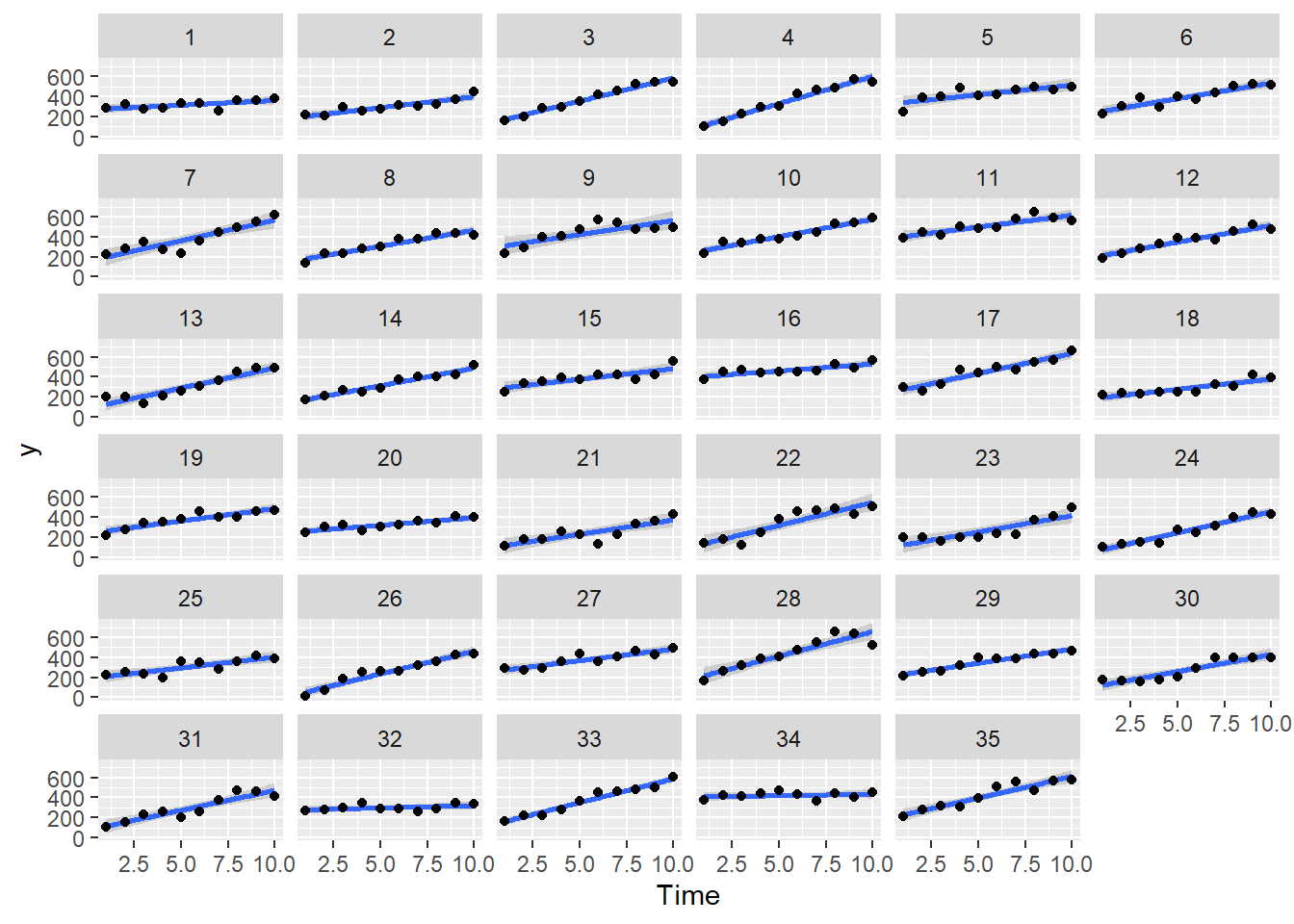
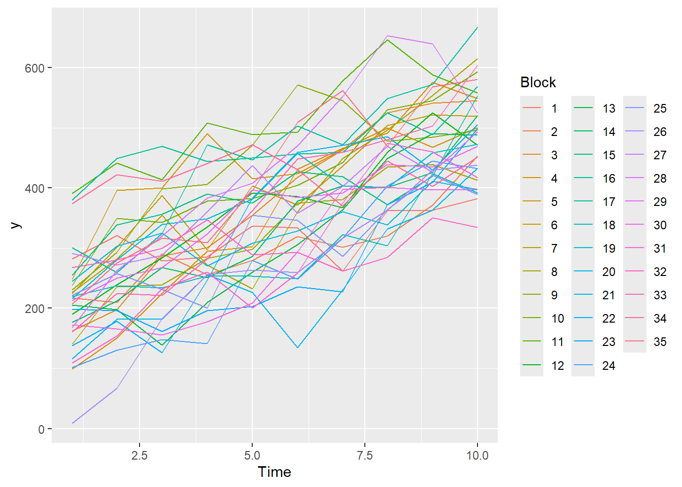
Imagine now that we has designed an experiment to investigate the effects of a continuous predictor (\(x\), for example time) on a response (\(y\)). Again, the system that we intend to sample is spatially heterogeneous and thus will add a great deal of noise to the data that will make it difficult to detect a signal (impact of treatment). Thus in an attempt to constrain this variability, we again decide to apply a design (RCB) in which each of the levels of \(X\) (such as time) treatments within each of \(35\) blocks dispersed randomly throughout the landscape. As this section is mainly about the generation of artificial data (and not specifically about what to do with the data), understanding the actual details are optional and can be safely skipped.
set.seed(123)slope <-30intercept <-200nBlock <-35nTime <-10sigma <-50sigma.block <-30n <- nBlock*nTimeBlock <-gl(nBlock, k=1)Time <-1:10rho <-0.8dt <-expand.grid(Time=Time,Block=Block)Xmat <-model.matrix(~-1+Block + Time, data=dt)block.effects <-rnorm(n = nBlock, mean = intercept, sd = sigma.block)#A.effects <- c(30,40)all.effects <-c(block.effects,slope)lin.pred <- Xmat %*% all.effects# ORXmat <-cbind(model.matrix(~-1+Block,data=dt),model.matrix(~Time,data=dt))## Sum to zero block effects##block.effects <- rnorm(n = nBlock, mean = 0, sd = sigma.block)###A.effects <- c(40,70,80)##all.effects <- c(block.effects,intercept,slope)##lin.pred <- Xmat %*% all.effects## the quadrat observations (within sites) are drawn from## normal distributions with means according to the site means## and standard deviations of 5eps <-NULLeps[1] <-0for (j in2:n) { eps[j] <- rho*eps[j-1] #residuals}y <-rnorm(n,lin.pred,sigma)+eps#OReps <-NULL# first value cant be autocorrelatedeps[1] <-rnorm(1,0,sigma)for (j in2:n) { eps[j] <- rho*eps[j-1] +rnorm(1, mean =0, sd = sigma) #residuals}y <- lin.pred + epsdata.rm <-data.frame(y=y, dt)head(data.rm) #print out the first six rows of the data set
NA          y Time Block
NA 1 282.1142    1     1
NA 2 321.1404    2     1
NA 3 278.7700    3     1
NA 4 285.8709    4     1
NA 5 336.6390    5     1
NA 6 333.5961    6     1
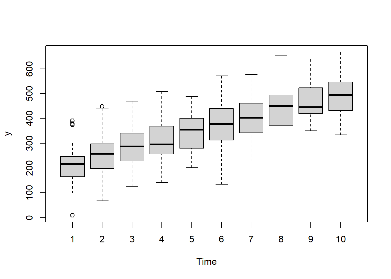
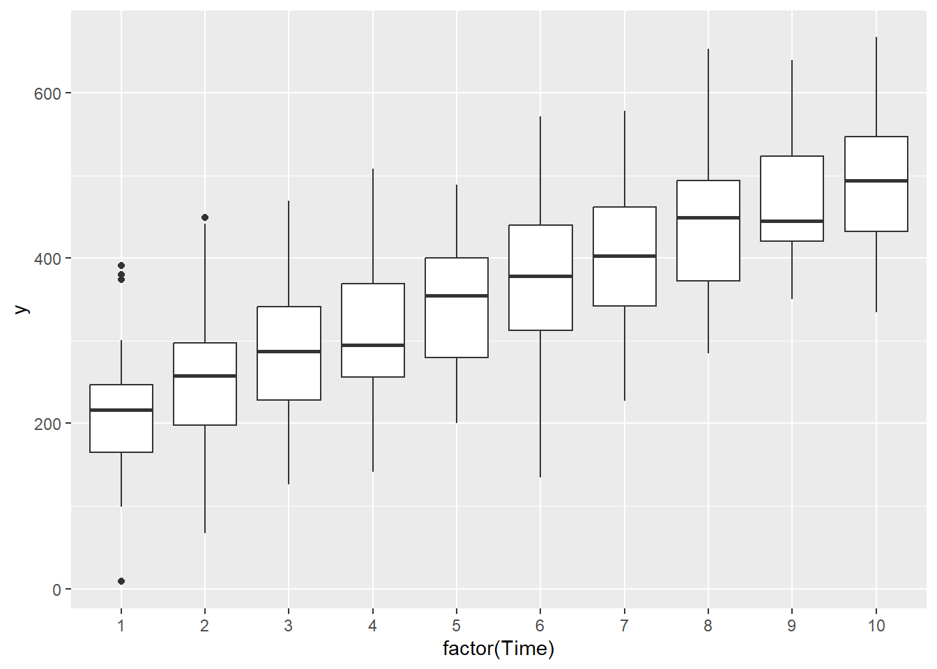
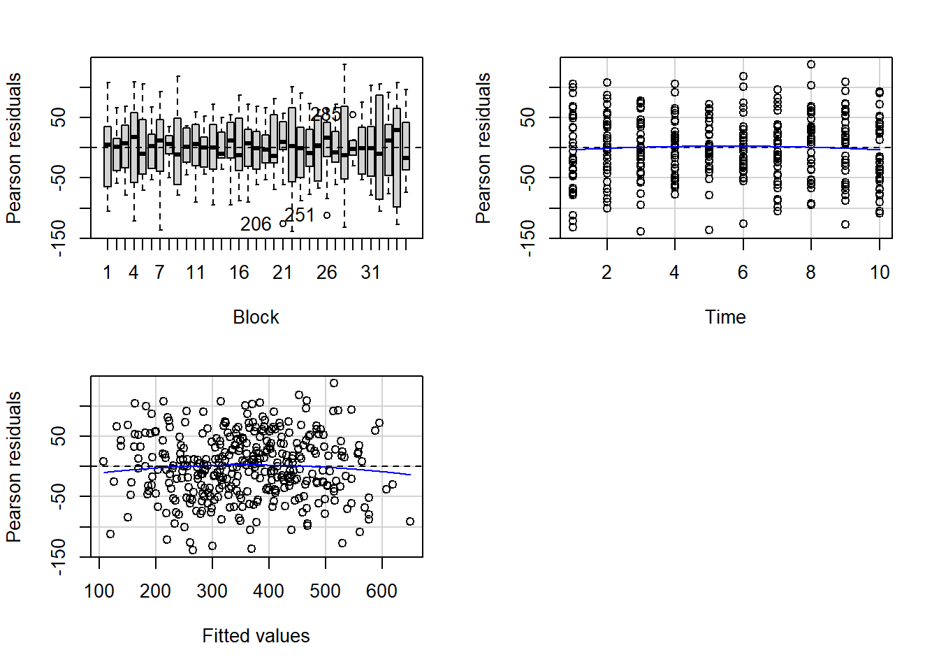
there is no evidence that the response variable is consistently non-normal across all populations - each boxplot is approximately symmetrical.
there is no evidence that variance (as estimated by the height of the boxplots) differs between the five populations. More importantly, there is no evidence of a relationship between mean and variance - the height of boxplots does not increase with increasing position along the \(y\)-axis. Hence it there is no evidence of non-homogeneity
Obvious violations could be addressed either by:
transform the scale of the response variables (to address normality, etc). Note transformations should be applied to the entire response variable (not just those populations that are skewed).
NA            Test stat Pr(>|Test stat|)
NA Block
NA Time         -0.7274           0.4675
NA Tukey test   -0.9809           0.3267
# the Tukey's non-additivity test by itself can be obtained via an internal function# within the car packagecar:::tukeyNonaddTest(lm(y~Block+Time, data.rm))
NA       Test     Pvalue
NA -0.9808606  0.3266615
# alternatively, there is also a Tukey's non-additivity test within the# asbio packagewith(data.rm,tukey.add.test(y,Time,Block))
NA
NA Tukey's one df test for additivity
NA F = 0.3997341   Denom df = 305    p-value = 0.5277003
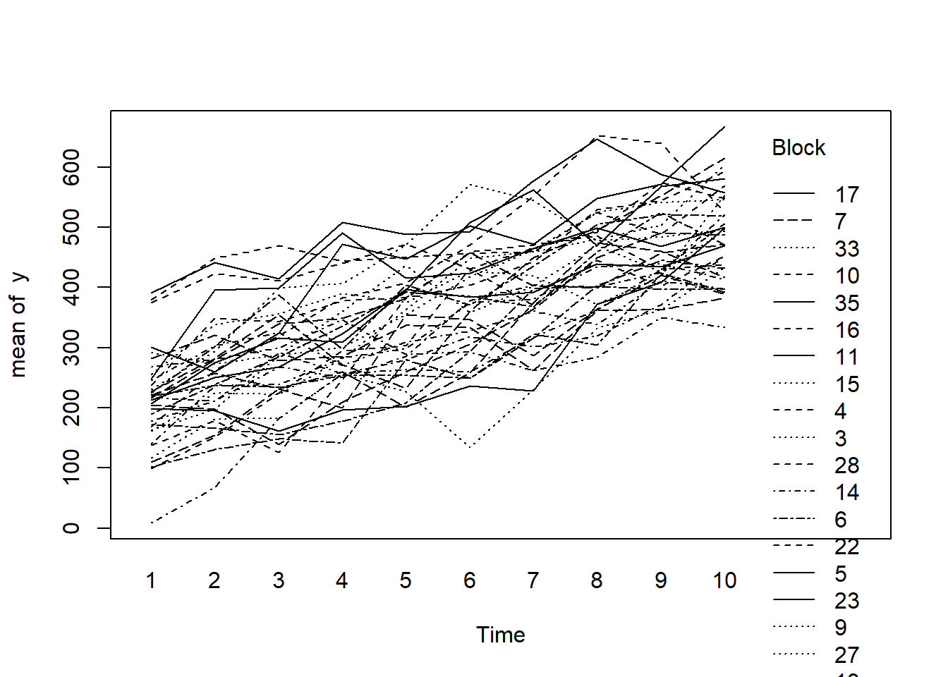
Conclusions:
there is no visual or inferential evidence of any major interactions between Block and the within-Block effect (Time). Any trends appear to be reasonably consistent between Blocks.
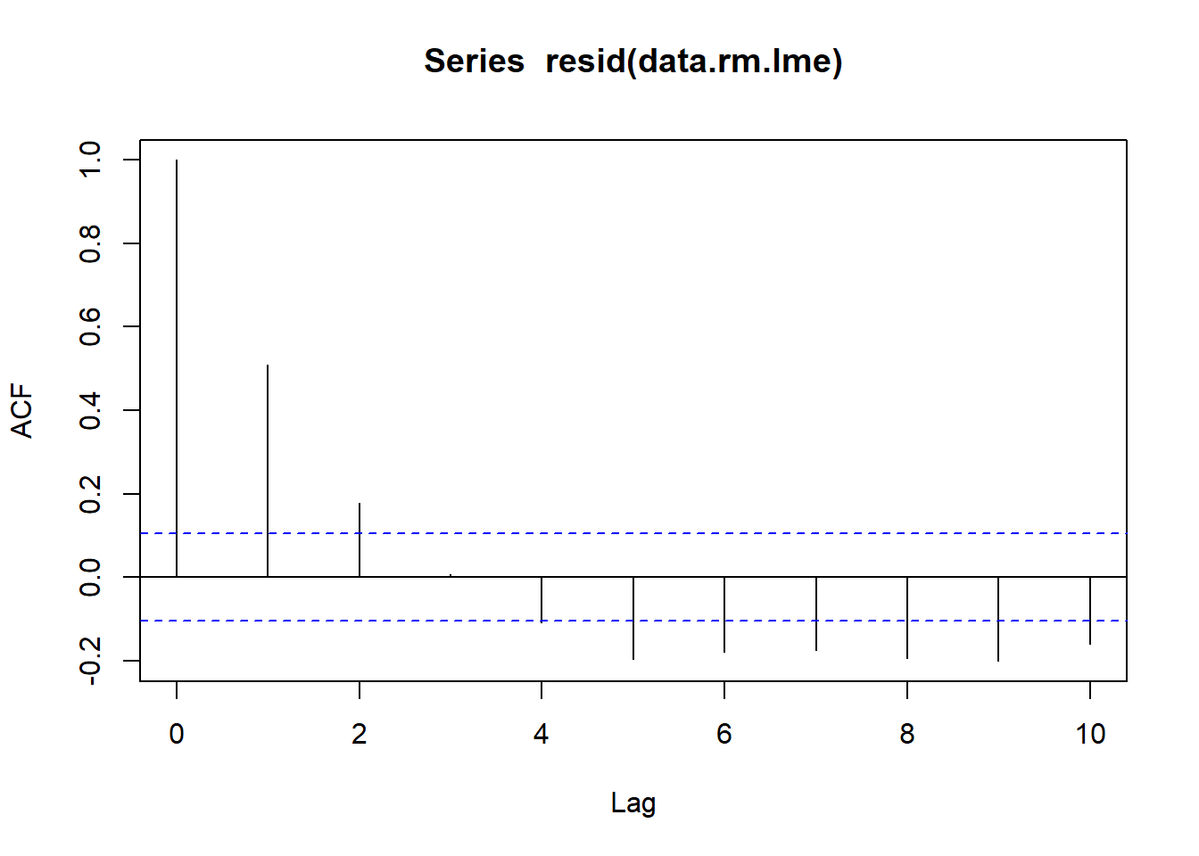
Sphericity
Since the levels of Time cannot be randomly assigned, it is likely that sphericity is not met. We can explore whether there is an auto-correlation patterns in the residuals. Note, as there was only ten time periods, it does not make logical sense to explore lags above \(10\).
The autocorrelation factor (ACF) at a range of lags up to \(10\), indicate that there is a cyclical pattern of residual auto-correlation. We really should explore incorporating some form of correlation structure into our model.
Model fitting
Matrix parameterisation
rstanString2="data{ int n; int nX; int nB; vector [n] y; matrix [n,nX] X; int B[n];}parameters{ vector [nX] beta; real<lower=0> sigma; vector [nB] gamma; real<lower=0> sigma_B;}transformed parameters { vector[n] mu; mu = X*beta; for (i in 1:n) { mu[i] = mu[i] + gamma[B[i]]; }} model{ // Priors beta ~ normal( 0 , 100 ); gamma ~ normal( 0 , sigma_B ); sigma_B ~ cauchy( 0 , 25 ); sigma ~ cauchy( 0 , 25 ); y ~ normal( mu , sigma );}"## write the model to a text filewriteLines(rstanString2, con ="matrixModel2.stan")Xmat <-model.matrix(~Time, data=data.rm)data.rm.list <-with(data.rm, list(y=y, X=Xmat, nX=ncol(Xmat),B=as.numeric(Block),n=nrow(data.rm), nB=length(levels(Block))))params <-c('beta','sigma','sigma_B')burnInSteps =3000nChains =2numSavedSteps =3000thinSteps =1nIter = burnInSteps+ceiling((numSavedSteps * thinSteps)/nChains)data.rm.rstan.d <-stan(data = data.rm.list, file ="matrixModel2.stan", chains = nChains, pars = params, iter = nIter, warmup = burnInSteps, thin = thinSteps)
NA
NA SAMPLING FOR MODEL 'anon_model' NOW (CHAIN 1).
NA Chain 1:
NA Chain 1: Gradient evaluation took 3e-05 seconds
NA Chain 1: 1000 transitions using 10 leapfrog steps per transition would take 0.3 seconds.
NA Chain 1: Adjust your expectations accordingly!
NA Chain 1:
NA Chain 1:
NA Chain 1: Iteration:    1 / 4500 [  0%]  (Warmup)
NA Chain 1: Iteration:  450 / 4500 [ 10%]  (Warmup)
NA Chain 1: Iteration:  900 / 4500 [ 20%]  (Warmup)
NA Chain 1: Iteration: 1350 / 4500 [ 30%]  (Warmup)
NA Chain 1: Iteration: 1800 / 4500 [ 40%]  (Warmup)
NA Chain 1: Iteration: 2250 / 4500 [ 50%]  (Warmup)
NA Chain 1: Iteration: 2700 / 4500 [ 60%]  (Warmup)
NA Chain 1: Iteration: 3001 / 4500 [ 66%]  (Sampling)
NA Chain 1: Iteration: 3450 / 4500 [ 76%]  (Sampling)
NA Chain 1: Iteration: 3900 / 4500 [ 86%]  (Sampling)
NA Chain 1: Iteration: 4350 / 4500 [ 96%]  (Sampling)
NA Chain 1: Iteration: 4500 / 4500 [100%]  (Sampling)
NA Chain 1:
NA Chain 1:  Elapsed Time: 1.194 seconds (Warm-up)
NA Chain 1:                0.285 seconds (Sampling)
NA Chain 1:                1.479 seconds (Total)
NA Chain 1:
NA
NA SAMPLING FOR MODEL 'anon_model' NOW (CHAIN 2).
NA Chain 2:
NA Chain 2: Gradient evaluation took 1.6e-05 seconds
NA Chain 2: 1000 transitions using 10 leapfrog steps per transition would take 0.16 seconds.
NA Chain 2: Adjust your expectations accordingly!
NA Chain 2:
NA Chain 2:
NA Chain 2: Iteration:    1 / 4500 [  0%]  (Warmup)
NA Chain 2: Iteration:  450 / 4500 [ 10%]  (Warmup)
NA Chain 2: Iteration:  900 / 4500 [ 20%]  (Warmup)
NA Chain 2: Iteration: 1350 / 4500 [ 30%]  (Warmup)
NA Chain 2: Iteration: 1800 / 4500 [ 40%]  (Warmup)
NA Chain 2: Iteration: 2250 / 4500 [ 50%]  (Warmup)
NA Chain 2: Iteration: 2700 / 4500 [ 60%]  (Warmup)
NA Chain 2: Iteration: 3001 / 4500 [ 66%]  (Sampling)
NA Chain 2: Iteration: 3450 / 4500 [ 76%]  (Sampling)
NA Chain 2: Iteration: 3900 / 4500 [ 86%]  (Sampling)
NA Chain 2: Iteration: 4350 / 4500 [ 96%]  (Sampling)
NA Chain 2: Iteration: 4500 / 4500 [100%]  (Sampling)
NA Chain 2:
NA Chain 2:  Elapsed Time: 1.21 seconds (Warm-up)
NA Chain 2:                0.283 seconds (Sampling)
NA Chain 2:                1.493 seconds (Total)
NA Chain 2:
print(data.rm.rstan.d , par =c('beta','sigma','sigma_B'))
NA Inference for Stan model: anon_model.
NA 2 chains, each with iter=4500; warmup=3000; thin=1;
NA post-warmup draws per chain=1500, total post-warmup draws=3000.
NA
NA           mean se_mean    sd   2.5%    25%    50%    75%  97.5% n_eff Rhat
NA beta[1] 186.70    0.72 11.96 162.54 178.89 186.74 194.88 209.68   272    1
NA beta[2]  30.79    0.02  1.02  28.82  30.10  30.77  31.48  32.75  2076    1
NA sigma    55.90    0.04  2.21  51.64  54.35  55.83  57.39  60.29  2729    1
NA sigma_B  64.52    0.19  8.76  50.39  58.35  63.49  69.44  83.96  2044    1
NA
NA Samples were drawn using NUTS(diag_e) at Mon Jul 22 12:09:12 2024.
NA For each parameter, n_eff is a crude measure of effective sample size,
NA and Rhat is the potential scale reduction factor on split chains (at
NA convergence, Rhat=1).
Given that Time cannot be randomized, there is likely to be a temporal dependency structure to the data. The above analyses assume no temporal dependency - actually, they assume that the variance-covariance matrix demonstrates a structure known as sphericity. Lets specifically model in a first order autoregressive correlation structure in an attempt to accommodate the expected temporal autocorrelation.
rstanString3="data{ int n; int nX; int nB; vector [n] y; matrix [n,nX] X; int B[n]; vector [n] tgroup;}parameters{ vector [nX] beta; real<lower=0> sigma; vector [nB] gamma; real<lower=0> sigma_B; real ar;}transformed parameters { vector[n] mu; vector[n] E; vector[n] res; mu = X*beta; for (i in 1:n) { E[i] = 0; } for (i in 1:n) { mu[i] = mu[i] + gamma[B[i]]; res[i] = y[i] - mu[i]; if(i>0 && i < n && tgroup[i+1] == tgroup[i]) { E[i+1] = res[i]; } mu[i] = mu[i] + (E[i] * ar); }} model{ // Priors beta ~ normal( 0 , 100 ); gamma ~ normal( 0 , sigma_B ); sigma_B ~ cauchy( 0 , 25 ); sigma ~ cauchy( 0 , 25 ); y ~ normal( mu , sigma );}"## write the model to a text filewriteLines(rstanString3, con ="matrixModel3.stan")Xmat <-model.matrix(~Time, data=data.rm)data.rm.list <-with(data.rm, list(y=y, X=Xmat, nX=ncol(Xmat),B=as.numeric(Block),n=nrow(data.rm), nB=length(levels(Block)),tgroup=as.numeric(Block)))params <-c('beta','sigma','sigma_B','ar')burnInSteps =3000nChains =2numSavedSteps =3000thinSteps =1nIter = burnInSteps+ceiling((numSavedSteps * thinSteps)/nChains)data.rm.rstan.d <-stan(data = data.rm.list, file ="matrixModel3.stan", chains = nChains, pars = params, iter = nIter, warmup = burnInSteps, thin = thinSteps)
NA
NA SAMPLING FOR MODEL 'anon_model' NOW (CHAIN 1).
NA Chain 1:
NA Chain 1: Gradient evaluation took 5.7e-05 seconds
NA Chain 1: 1000 transitions using 10 leapfrog steps per transition would take 0.57 seconds.
NA Chain 1: Adjust your expectations accordingly!
NA Chain 1:
NA Chain 1:
NA Chain 1: Iteration:    1 / 4500 [  0%]  (Warmup)
NA Chain 1: Iteration:  450 / 4500 [ 10%]  (Warmup)
NA Chain 1: Iteration:  900 / 4500 [ 20%]  (Warmup)
NA Chain 1: Iteration: 1350 / 4500 [ 30%]  (Warmup)
NA Chain 1: Iteration: 1800 / 4500 [ 40%]  (Warmup)
NA Chain 1: Iteration: 2250 / 4500 [ 50%]  (Warmup)
NA Chain 1: Iteration: 2700 / 4500 [ 60%]  (Warmup)
NA Chain 1: Iteration: 3001 / 4500 [ 66%]  (Sampling)
NA Chain 1: Iteration: 3450 / 4500 [ 76%]  (Sampling)
NA Chain 1: Iteration: 3900 / 4500 [ 86%]  (Sampling)
NA Chain 1: Iteration: 4350 / 4500 [ 96%]  (Sampling)
NA Chain 1: Iteration: 4500 / 4500 [100%]  (Sampling)
NA Chain 1:
NA Chain 1:  Elapsed Time: 1.438 seconds (Warm-up)
NA Chain 1:                0.502 seconds (Sampling)
NA Chain 1:                1.94 seconds (Total)
NA Chain 1:
NA
NA SAMPLING FOR MODEL 'anon_model' NOW (CHAIN 2).
NA Chain 2:
NA Chain 2: Gradient evaluation took 2.7e-05 seconds
NA Chain 2: 1000 transitions using 10 leapfrog steps per transition would take 0.27 seconds.
NA Chain 2: Adjust your expectations accordingly!
NA Chain 2:
NA Chain 2:
NA Chain 2: Iteration:    1 / 4500 [  0%]  (Warmup)
NA Chain 2: Iteration:  450 / 4500 [ 10%]  (Warmup)
NA Chain 2: Iteration:  900 / 4500 [ 20%]  (Warmup)
NA Chain 2: Iteration: 1350 / 4500 [ 30%]  (Warmup)
NA Chain 2: Iteration: 1800 / 4500 [ 40%]  (Warmup)
NA Chain 2: Iteration: 2250 / 4500 [ 50%]  (Warmup)
NA Chain 2: Iteration: 2700 / 4500 [ 60%]  (Warmup)
NA Chain 2: Iteration: 3001 / 4500 [ 66%]  (Sampling)
NA Chain 2: Iteration: 3450 / 4500 [ 76%]  (Sampling)
NA Chain 2: Iteration: 3900 / 4500 [ 86%]  (Sampling)
NA Chain 2: Iteration: 4350 / 4500 [ 96%]  (Sampling)
NA Chain 2: Iteration: 4500 / 4500 [100%]  (Sampling)
NA Chain 2:
NA Chain 2:  Elapsed Time: 2.343 seconds (Warm-up)
NA Chain 2:                0.483 seconds (Sampling)
NA Chain 2:                2.826 seconds (Total)
NA Chain 2:
print(data.rm.rstan.d , par =c('beta','sigma','sigma_B','ar'))
NA Inference for Stan model: anon_model.
NA 2 chains, each with iter=4500; warmup=3000; thin=1;
NA post-warmup draws per chain=1500, total post-warmup draws=3000.
NA
NA           mean se_mean    sd   2.5%    25%    50%    75%  97.5% n_eff Rhat
NA beta[1] 179.17    0.24 12.76 153.91 170.91 179.06 187.48 204.24  2816    1
NA beta[2]  31.29    0.02  1.70  27.91  30.17  31.29  32.43  34.72  5406    1
NA sigma    48.73    0.03  1.99  45.11  47.33  48.63  50.06  52.72  5115    1
NA sigma_B  49.78    0.26 10.61  30.48  42.28  49.07  56.56  73.10  1604    1
NA ar        0.78    0.00  0.05   0.68   0.75   0.78   0.81   0.88  2786    1
NA
NA Samples were drawn using NUTS(diag_e) at Mon Jul 22 12:09:49 2024.
NA For each parameter, n_eff is a crude measure of effective sample size,
NA and Rhat is the potential scale reduction factor on split chains (at
NA convergence, Rhat=1).
References
Gelman, Andrew, Daniel Lee, and Jiqiang Guo. 2015. “Stan: A Probabilistic Programming Language for Bayesian Inference and Optimization.”Journal of Educational and Behavioral Statistics 40 (5): 530–43.
Stan Development Team. 2018. “RStan: The R Interface to Stan.”http://mc-stan.org/.