Introduction
Up until now (in the proceeding tutorials), the focus has been on models that adhere to specific assumptions about the underlying populations (and data). Indeed, both before and immediately after fitting these models, I have stressed the importance of evaluating and validating the proposed and fitted models to ensure reliability of the models. It is now worth us revisiting those fundamental assumptions as well as exploring the options that are available when the populations (data) do not conform. Let’s explore a simple linear regression model to see how each of the assumptions relate to the model.
\[
y_i = \beta_0 + \beta_1x_i + \epsilon_i \;\;\; \text{with} \;\;\; \epsilon_i \sim \text{Normal}(0, \sigma^2).
\]
The above simple statistical model models the linear relationship of \(y_i\) against \(x_i\). The residuals (\(\epsilon\)) are assumed to be normally distributed with a mean of zero and a constant (yet unknown) variance (\(\sigma\), homogeneity of variance). The residuals (and thus observations) are also assumed to all be independent.
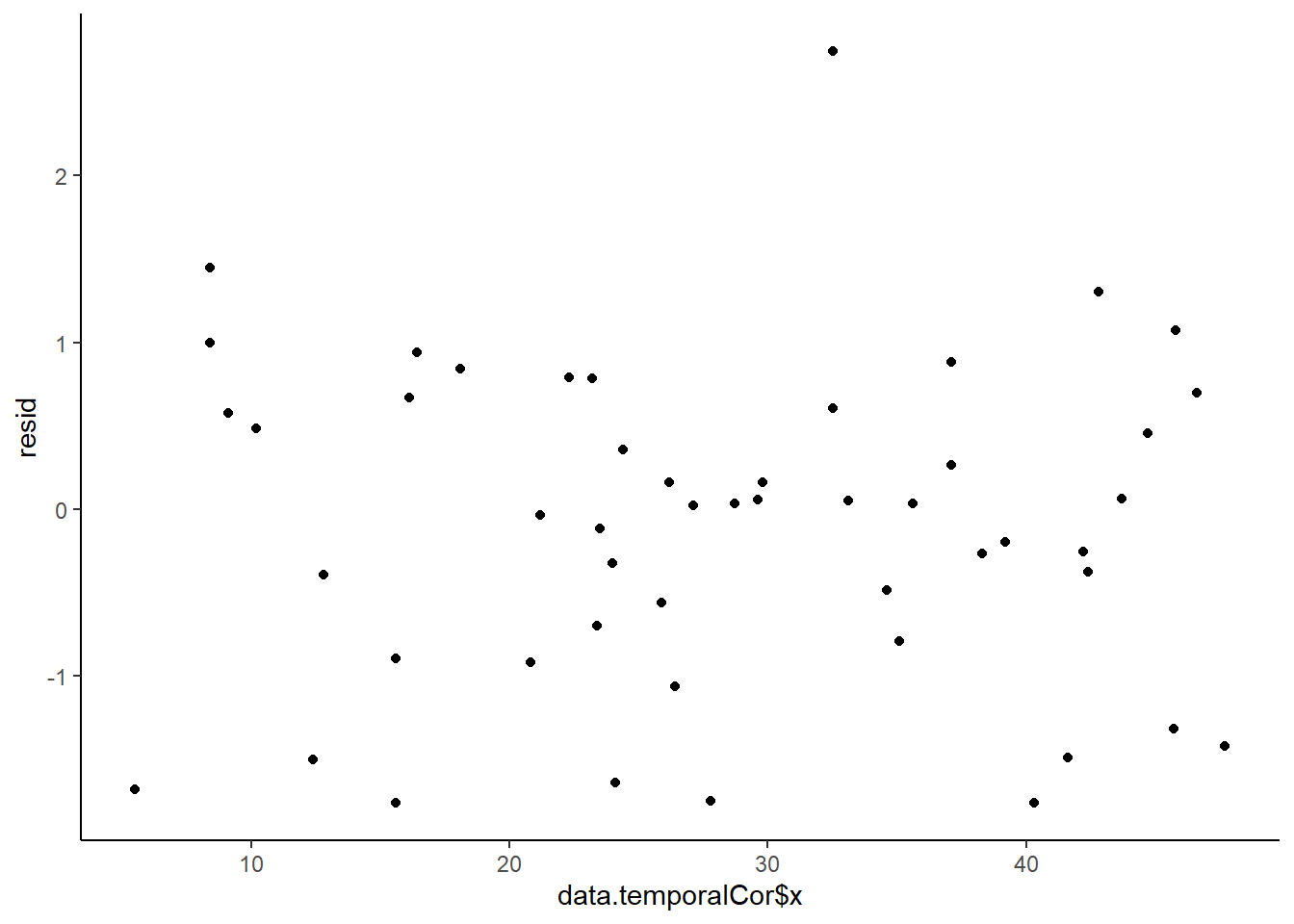
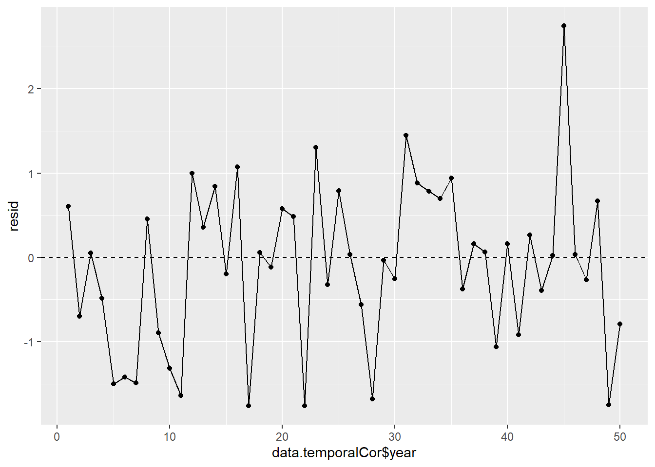
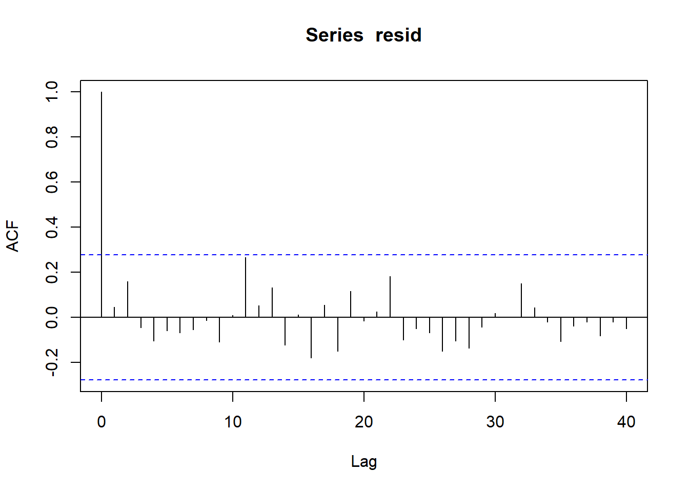
Homogeneity of variance and independence are encapsulated within the single symbol for variance (\(\sigma^2\)). In assuming equal variances and independence, we are actually making an assumption about the variance-covariance structure of the populations (and thus residuals). Specifically, we assume that all populations are equally varied and thus can be represented well by a single variance term (all diagonal values in a \(N\times N\) covariance matrix are the same, \(\sigma^2\)) and the covariances between each population are zero (off diagonals). In simple regression, each observation (data point) represents a single observation drawn (sampled) from an entire population of possible observations. The above covariance structure thus assumes that the covariance between each population (observation) is zero - that is, each observation is completely independent of each other observation. Whilst it is mathematically convenient when data conform to these conditions (normality, homogeneity of variance, independence and linearity), data often violate one or more of these assumptions. In the following, I want to discuss and explore the causes and options for dealing with non-compliance to each of these conditions. By gaining a better understanding of how the various model fitting engines perform their task, we are better equipped to accommodate aspects of the data that don’t otherwise conform to the simple regression assumptions. In this tutorial we specifically focus on the topic of heterogeneity of the variance.
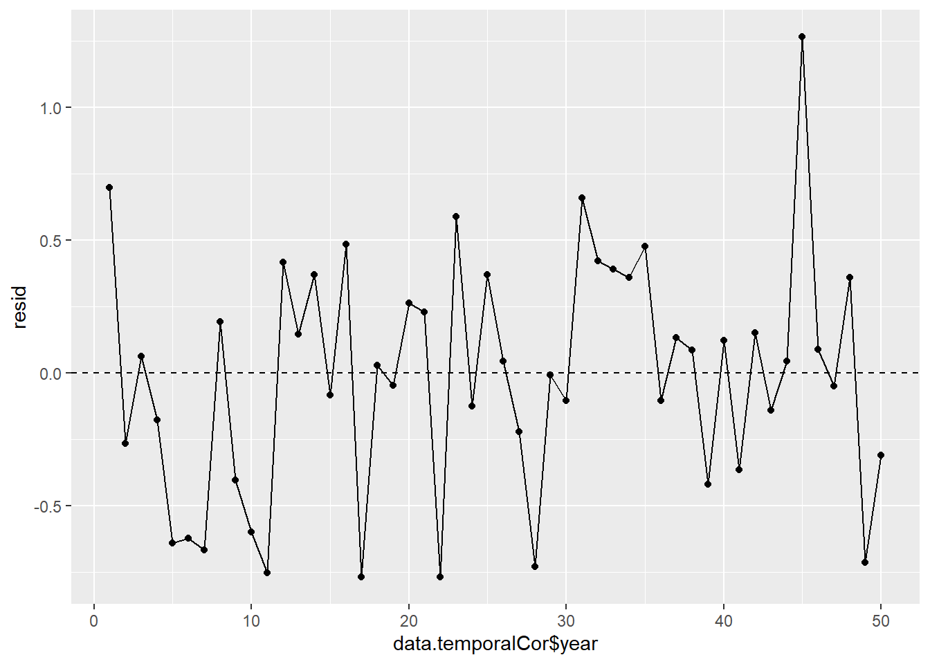
In order that the estimated parameters represent the underlying populations in an unbiased manner, the residuals (and thus each each observation) must be independent. However, what if we were sampling a population over time and we were interested in investigating how changes in a response relate to changes in a predictor (such as rainfall). For any response that does not “reset” itself on a regular basis, the state of the population (the value of its response) at a given time is likely to be at least partly dependent on the state of the population at the sampling time before. We can further generalise the above into:
\[
y_i \sim Dist(\mu_i),
\]
where \(\mu_i=\boldsymbol X \boldsymbol \beta + \boldsymbol Z \boldsymbol \gamma\), with \(\boldsymbol X\) and \(\boldsymbol \beta\) representing the fixed data structure and fixed effects, respectively, while with \(\boldsymbol Z\) and \(\boldsymbol \gamma\) represent the varying data structure and varying effects, respectively. In simple regression, there are no “varying” effects, and thus:
\[
\boldsymbol \gamma \sim MVN(\boldsymbol 0, \boldsymbol \Sigma),
\]
where \(\boldsymbol \Sigma\) is a variance-covariance matrix of the form
\[
\boldsymbol \Sigma = \frac{\sigma^2}{1-\rho^2}
\begin{bmatrix}
1 & \rho^{\phi_{1,2}} & \ldots & \rho^{\phi_{1,n}} \\
\rho^{\phi_{2,1}} & 1 & \ldots & \vdots\\
\vdots & \ldots & 1 & \vdots\\
\rho^{\phi_{n,1}} & \ldots & \ldots & 1
\end{bmatrix}.
\]
Notice that this introduces a very large number of additional parameters that require estimating: \(\sigma^2\) (error variance), \(\rho\) (base autocorrelation) and each of the individual covariances (\(\rho^{\phi_{n,n}}\)). Hence, there are always going to be more parameters to estimate than there are date avaiable to use to estimate these paramters. We typically make one of a number of alternative assumptions so as to make this task more manageable.
- When we assume that all residuals are independent (regular regression), i.e. \(\rho=0\), \(\boldsymbol \Sigma\) is essentially equal to \(\sigma^2 \boldsymbol I\) and we simply use:
\[
\boldsymbol \gamma \sim N( 0,\sigma^2).
\]
- We could assume there is a reasonably simple pattern of correlation that declines over time. The simplest of these is a first order autoregressive (AR1) structure in which exponent on the correlation declines linearly according to the time lag (\(\mid t - s\mid\)).
\[
\boldsymbol \Sigma = \frac{\sigma^2}{1-\rho^2}
\begin{bmatrix}
1 & \rho & \ldots & \rho^{\mid t-s \mid} \\
\rho & 1 & \ldots & \vdots\\
\vdots & \ldots & 1 & \vdots\\
\rho^{\mid t-s \mid } & \ldots & \ldots & 1
\end{bmatrix}.
\]
Note, in making this assumption, we are also assuming that the degree of correlation is dependent only on the lag and not on when the lag occurs (stationarity). That is all lag 1 residual pairs will have the same degree of correlation, all the lag \(2\) pairs will have the same correlation and so on.