Conducting trial-based cost-effectiveness analyses:

A tutorial

Author

Affiliation

Andrea Gabrio

Maastricht University

Hello folks, I hope you are well and welcome back to my blog. Today, after taking a break from HTA in the past posts, I would like to resume one of my favourite topics: statistical methods for cost-effectiveness analyses. One of the reasons that pushed me to cover once more this topic is the fact that I will shortly give a presentation about this within my university with the objective to highlight the current state of play in the field. I would like then to take this opportunity (otherwise it could take a long time for me to organise my code again) to provide here a short summary of the different elements I will touch in my talk. Perhaps I will need to split the topics in two posts as the amount of things that will be discussed is quite a lot, but I am not sure yet about this. Let’s see how it goes.

For now, I just want to introduce the topic and put out the disclaimer that, given that I will mostly focus on typical methods used in trial-based analyses, I will strictly focus on frequentist methods and their implementation using standard R functions and packages. Thus, no Bayesian methods will be discussed/coded today, unfortunately! But no worries, there will be plenty of time to discuss Bayesian methods for HTA in the future. Actually, if interested, a new book for which I also collaborated has been recently published (Baio, Thom, and Pechlivanoglou 2025) which I highly recommend if you want to have a more in-depth look at how to code advanced methods for HTA in R, including Bayesian! The chapter I coordinated and written is the one on missing data (I believe chapter 3?), naturally. I think you will find very helpful if you are too scared about statistics and programming (I promise that things are not that difficult and everything is well described and illustrated).

Moving on, let’s get into the content of today’s post! The focus will be around the typical complexities that affect trial-based CE data and what has been done and is currently recommended in the literature to deal with them when conducting the analyses. I will also partly follow the structure and order of topics discussed in a relatively recent review (El Alili et al. 2022), which I strongly recommend to look at for references. Given the limited available, I will focus on those methods and issues that are directly mentioned in the recent national guidelines from the Dutch HTA agency ZorgInstituut Nederland(Nederland 2024) about the statistical analysis of (empirical) trial-based health economic evaluations in the Netherlands. In particular, I will focus on the following aspects:

• Imbalances in mean baseline effects/costs between arms, if not accounted for, may distort CE results(Manca, Hawkins, and Sculpher 2005; Van Asselt et al. 2009)

• Ignoring the correlation between effects & costs is inappropriate and will lead to a loss in efficiency for the estimates (Willan, Briggs, and Hoch 2004)

• Skewness} in effects/costs in small samples undermines the validity of asymptotic tests and may lead to incorrect results (J. A. Barber and Thompson 2000)

• Clustering of data linked to treatment (eg cluster RCTs) invalidates the assumptions of standard methods (eg OLS), underestimates variance and possibly bias results (Gomes, Ng, et al. 2012)

• Missing effects/costs during follow-up are common and may introduce bias. Methods that appropriately account for missing data uncertainty and assess the sensitivity of results are needed (Gabrio, Mason, and Baio 2017; Leurent, Gomes, and Carpenter 2018)

Regression Adjustment for Baseline Imbalances

We start by considering the problem of the possible occurrence of some imbalances between treatment arms in some baseline variables. In the context of randomised trial-based CUAs, a typical example of these variables are baseline utilities (Manca, Hawkins, and Sculpher 2005) or costs (Van Asselt et al. 2009). Despite randomisation, some baseline imbalances are likely to occur, especially in those baseline variables that are likely strongly associated with the main outcomes of interest for the analysis, i.e. QALYs and Total Costs. This is a particular issue for baseline utilities, which are directly used in the calculation of QALYs through the Area Under the Curve (AUC) method (Drummond et al. 2015). If these imbalances are not adjusted for, estimates from the main analysis are likely to be affected (eg mean QALY difference or ICER estimates), especially in the event of substantial differences, and possibly lead to misleading CE conclusions.

Data generation

The following (folded) code is simply used to generate some artificial CEA data for exemplary purposes to demonstrate how regression adjustment may be conducted in R. If not of interest, you may skip the folded code and jump to the actual implementation code in the next section.

#generate multivariate trial CUA data (utilities)
library(mvtnorm) #load library to generate multivariate normal data
n0 <- n1 <- 2000 #sample size for control (0) and new trt (1)
time <- 3 #n of time points

#mean utilities at each time in control
mu0 <- c(0.63,0.63,0.67) 
#covariance matrix for utilities in control
Sigma0 <- diag(3)  
diag(Sigma0) <- c(0.1^2,0.1^2,0.1^2)
rho0 <- 0.85 #correlation across time in control
Sigma0[1,2] <- Sigma0[2,1] <- rho0*0.1*0.1
Sigma0[3,1] <- Sigma0[1,3] <- rho0*0.1*0.1
Sigma0[3,2] <- Sigma0[2,3] <- rho0*0.1*0.1
#mean utilities at each time in new trt
mu1 <- c(0.55,0.63,0.67) 
Sigma1 <- diag(3) 
diag(Sigma1) <- c(0.1^2,0.1^2,0.1^2) 
rho1 <- 0.85 #correlation across time in new trt
#covariance matrix for utilities in new trt
Sigma1[1,2] <- Sigma1[2,1] <- rho1*0.1*0.1
Sigma1[3,1] <- Sigma1[1,3] <- rho1*0.1*0.1
Sigma1[3,2] <- Sigma1[2,3] <- rho1*0.1*0.1

#set rng seed for reproducibility
set.seed(2345)
#simulate data by arm
u0 <- rmvnorm(n0, mean = mu0, sigma = Sigma0)
u1 <- rmvnorm(n1, mean = mu1, sigma = Sigma1)
#compute QALYs via AUC by arm
QALY0 <- ((u0[,1]+u0[,2])/2)*(6/12) + ((u0[,2]+u0[,3])/2)*(6/12)
QALY1 <- ((u1[,1]+u1[,2])/2)*(6/12) + ((u1[,2]+u1[,3])/2)*(6/12)

#rename variables and create dataset
u_base <- c(u0[,1],u1[,1])
u_6m <- c(u0[,2],u1[,2])
u_12m <- c(u0[,3],u1[,3])
QALY <- c(QALY0, QALY1)
trt <- c(rep("old",n0),rep("new",n1))
dataset <- data.frame(u_base,u_6m,u_12m,QALY,trt)
#make trt a factor variable (old,new)
dataset$trt <- factor(trt, levels = c("old", "new"))
#randomly shuffle rows of the dataset
dataset <- dataset[sample(1:nrow(dataset)), ]

We can inspect the first few rows of the generated data stored in the R object dataset, for example by typing the following command

head(dataset, n=8)

        u_base      u_6m     u_12m      QALY trt
1851 0.6649710 0.6695179 0.6385095 0.6606291 old
3885 0.5024305 0.6252957 0.6733950 0.6066042 new
2100 0.5250719 0.6123696 0.6940127 0.6109560 new
1430 0.6435694 0.6345586 0.6374612 0.6375370 old
2705 0.4929146 0.5621082 0.5388496 0.5389951 new
2774 0.6824814 0.7805227 0.8651590 0.7771715 new
537  0.5938100 0.5543479 0.6344838 0.5842474 old
3667 0.4878960 0.5223296 0.6684593 0.5502536 new

which shows for a few rows (individuals) their related values for the following hypothetical variables: baseline utility, 6 and 12 months follow-up utility, QALY and treatment allocation.

Method application

Regression adjustment is a technique which allows to obtained estimates of parameters of interest, i.e. mean QALY differential \(\Delta_e=\text{E}[\text{QALY}\mid \text{New}]-\text{E}[\text{QALY}\mid \text{old}]\), while also controlling for possible imbalances in some baseline variables. Although alternative adjustment methods exist, regression-based adjustment is by far the most popular and recommended in the literature since it can be easily implemented and can provide valid adjusted estimates with respect to multiple baseline variables (Manca, Hawkins, and Sculpher 2005).

Usually, estimates for \(\Delta_e\) are retrieved after fitting a standard Ordinary Least Square (OLS) linear regression to QALYs using the treatment arm indicator as the key independent variable into the model.

\[ \text{QALY}_i = \beta_0+\beta_1\times \text{arm}_i + \varepsilon_i \tag{1}\]

where \(\text{QALY}_i\) and \(\text{arm}_i\) denote the outcome and treatment indicator value for individual \(i=1,\ldots,N\) in the trial, while \(\varepsilon_i\) denote the individual-level error term assumed to follow a Normal distribution with mean \(0\) and variance \(\sigma^2\).

Estimates of the regression coefficients \(\hat{\beta}=(\hat{\beta}_0,\hat{\beta}_1)\) in Equation 1 can then be used to derive the unadjusted mean QALYs in each treatment group

\[ \begin{aligned} \text{E}[\text{QALY}\mid \text{arm}=\text{old}] &= \hat{\beta}_0\\ \text{E}[\text{QALY}\mid \text{arm}=\text{new}] &= \hat{\beta}_0+\hat{\beta}_1,\\ \end{aligned} \] with \(\hat{\beta}_1\) representing the mean difference between the reference group (eg New) with respect to the comparator (eg Old).

Adjustment for some baseline variable, eg baseline utilities \(u_{i0}\), can be easily achieved by including the corresponding baseline variable into the regression as an additional independent variable. Thus, the model regression becomes

\[ \text{QALY}_i = \beta_0+\beta_1\times \text{arm}_i + \beta_2\times \text{u}_{i0}+ \varepsilon_i \tag{2}\]

where \(\hat{\beta}_2\) represents the coefficient associated with \(u_{i0}\) (ie how much QALY changes for a unit change in baseline utility). By simply including \(u_{i0}\) into the model, adjusted estimates for \(\hat{\beta}_1\) from Equation 2 can be obtained in a similar way to the unadjusted model. The only difference is in case we need to estimate mean QALYs in each treatment group:

\[ \begin{aligned} \text{E}[\text{QALY}\mid \text{arm}=\text{old}] &= \hat{\beta}_0+\hat{\beta}_2\times \bar{\text{u}}_{0}\\ \text{E}[\text{QALY}\mid \text{arm}=\text{new}] &= \hat{\beta}_0+\hat{\beta}_1+\hat{\beta}_2\times \bar{\text{u}}_{0},\\ \end{aligned} \tag{3}\]

which can be obtained after setting the value of \(\text{u}_{i0}\) to its sample mean across treatment groups (denoted with \(\bar{\text{u}}_{0}\)).

Now, let’s all do this in R. First, let’s fit the adjusted model and summarise the output

#fit OLS regression adjusting for baseline utility
lm_adj <- lm(QALY ~ trt + u_base, data = dataset)
#summarise output
summary(lm_adj)

Call:
lm(formula = QALY ~ trt + u_base, data = dataset)

Residuals:
      Min        1Q    Median        3Q       Max 
-0.133578 -0.023659 -0.000639  0.023359  0.116394 

Coefficients:
            Estimate Std. Error t value Pr(>|t|)    
(Intercept) 0.084463   0.003556   23.75   <2e-16 ***
trtnew      0.051304   0.001178   43.56   <2e-16 ***
u_base      0.880692   0.005528  159.31   <2e-16 ***
---
Signif. codes:  0 '***' 0.001 '**' 0.01 '*' 0.05 '.' 0.1 ' ' 1

Residual standard error: 0.03454 on 3997 degrees of freedom
Multiple R-squared:  0.8653,    Adjusted R-squared:  0.8652 
F-statistic: 1.284e+04 on 2 and 3997 DF,  p-value: < 2.2e-16

We can see in the coefficients “Estimate” column the values for: \(\hat{\beta}_0=0.084\), \(\hat{\beta}_1=0.051\) and \(\hat{\beta}_2=0.881\). In addition, we can also find the value for the “Residual standard error” \(\sigma=0.035\).

In the following (folded) code part I will show how to manually compute the estimates in Equation 3 based on the regression output.

#extract regression coefficients
betas <- coef(lm_adj)
#extract error standard deviation
sigma <- summary(lm_adj)$sigma
#extract all independent variables
Xs <- model.matrix(lm_adj)
#compute matrix multiplication 
XtX.inv <- solve(t(Xs) %*% Xs) 
#select profile to be estimated in terms of: intercept, trt, u_base
prof_old <- c(1,0,mean(dataset$u_base)) #1=intercept,0=trt,u_base=mean(u)
prof_new <- c(1,1,mean(dataset$u_base)) #1=intercept,1=trt,u_base=mean(u)
#compute linear combination of regression parameters
mean_old <- betas["(Intercept)"] + betas["u_base"]*mean(dataset$u_base)
mean_new <- betas["(Intercept)"] + betas["trtnew"] + betas["u_base"]*mean(dataset$u_base)
#compute associated standard errors
std.err_old <- sigma * sqrt(t(prof_old) %*% XtX.inv %*% prof_old)
std.err_new <- sigma * sqrt(t(prof_new) %*% XtX.inv %*% prof_new)
#compute associated confidence intervals 
alpha<-0.05 #95% CI
n <- dim(dataset)[1] #total sample size
df <- n-c(length(betas)-1) #degrees of freedom
t.critic <- qt(1-alpha/2,df=df) #critical value for t distribution and 95% CI
mean_old_lower.CI <- mean_old - t.critic*std.err_old
mean_old_upper.CI <- mean_old + t.critic*std.err_old
mean_new_lower.CI <- mean_new - t.critic*std.err_new
mean_new_upper.CI <- mean_new + t.critic*std.err_new
#combine all results
mean_old_summary <- c(mean_old,std.err_old,mean_old_lower.CI,mean_old_upper.CI)
mean_new_summary <- c(mean_new,std.err_new,mean_new_lower.CI,mean_new_upper.CI)
#attach names to each value
names(mean_old_summary) <- c("Estimate","SE","CI(low)","CI(high)")
names(mean_new_summary) <- c("Estimate","SE","CI(low)","CI(high)")

We can also rely on the pre-built function emmean from the R package emmeans to compute the mean QALYs in each treatment group in a more automatic way. For example, we can type the following

library(emmeans) #load library to obtain marginal means
lm_adj_em <- emmeans(lm_adj, ~ trt) #compute mean outcome by level of trt
lm_adj_em

 trt emmean       SE   df lower.CL upper.CL
 old 0.6023 0.000803 3997   0.6007   0.6039
 new 0.6536 0.000803 3997   0.6520   0.6552

Confidence level used: 0.95 

to directly obtain estimates of the mean QALYs, their standard errors and \(95\%\) confidence intervals by treatment group (hopefully they are the same as those computed manually before!). In addition, it is also possible to use the function contrast to derive estimates of any linear combination of the quantities above. For example, we may obtain estimates for the mean QALY difference (New - Old) by typing

#take difference as - Old + New = New - Old
QALY_new_vs_old <- list("New vs Old" = c(-1, 1))
#compute linear combination
lm_adj_em_delta_e <- contrast(lm_adj_em, QALY_new_vs_old) 
#obtain results in terms of confidence intervals
confint(lm_adj_em_delta_e, level = 0.95)

 contrast   estimate      SE   df lower.CL upper.CL
 New vs Old   0.0513 0.00118 3997    0.049   0.0536

Confidence level used: 0.95 

Although I have not shown here an application of regression adjustment to control for baseline costs when deriving Total Costs mean and mean differential estimates, these can be easily obtained in a similar way to what shown for QALYs and baseline utilities. In the following sections I will show how these computations can be embedded within a bootstrapping procedure for both outcome variables and how to obtain bootstrapped estimates for the quantities of interest for the CEA.

Summary

In general, it is good to keep in mind the following features when implementing regression-based adjustment:

• Advantages:

  • Easy to implement
  • Allow to control for multiple variables
  • Assess impact of specific variables on marginal CE outcomes (eg via interaction terms)

• Drawbacks:

  • Assume variables’ distribution is the same across arms
  • Adjusting for many variables may result in “overfitting”

There are also alternatives to regression-based adjustment, although these have been less used in the CEA literature and have their own advantages and drawbacks. Examples include: Propensity score adjustment (Indurkhya, Mitra, and Schrag 2006), Propensity Score Matching & Genetic Matching (Sekhon and Grieve 2012)

Correlation between CE outcomes

A typical feature of trial-based CE data is the presence of some form of correlation between the effect and cost variables. This may happen because: new treatments come from intensive research and are positively associated with higher unit costs, or new treatments negatively affect care pathway costs (eg fewer hospitalisations, side effects, etc.). When this association, either positive or negative, is substantial, simply running separate OLS models for each outcome (as in Section 1) will provide inefficient estimates in the sense that the level of uncertainty around the parameter estimates will be overestimated, thus resulting in higher standard errors and wider confidence intervals.

To address this problem, joint modelling of both outcome variables is typically recommended to properly characterise the level of uncertainty around parameter estimates and CE results (O’Hagan and Stevens 2001). Indeed, by simultaneously modelling both outcomes within a multivariate analysis it is possible to borrow information across variables to estimate variance components and standard errors more efficiently with respect to separate univariate analyses. A general issue, however, is that multivariate modelling, while also allowing for regression adjustment for each outcome separately (ie using different baseline variables per outcome), is not straightforward to implement using standard software packages, especially wihtin a frequentist statistical framework.

To overcome this practical issue, correlation between outcomes can also be taken into account using alternative approaches, which have become increasingly popular in trial-based CEA. These include: Seemingly Unrelated Regression (SUR) equations framework (Willan, Briggs, and Hoch 2004), (non-parametric) bootstrapping procedure (Nixon, Wonderling, and Grieve 2010), or even a combination of these two methods.

Data generation

As usual, let’s start by generating some artificial data that will be used to show how to implement the methods in R. The code used to generate these data is provided in the following (folded) code part and, if not of interest, you may skip it and jump to the actual implementation code in the next section.

#remove scientific notation to be displayed by R
options(scipen=999) 
#generate data
library(mvtnorm) #load package to generate multivariate normal data
n0 <- n1 <- 150 #arm-specific sample sizes (0=old,1=new)
mu0 <- c(0.58,3) #mean QALY and TC in old arm
#2x2 Covariance matrix for QALY and TC in old arm
Sigma0 <- diag(2) 
diag(Sigma0) <- c(0.1^2,1^2) #set variances for each outcome in old arm
rho0 <- 0.75 #set correlation between outcomes in old arm
Sigma0[1,2] <- Sigma0[2,1] <- rho0*0.1*1 #set covariances in old arm
#do the same for new arm
mu1 <- c(0.65,3)
Sigma1 <- diag(2) 
diag(Sigma1) <- c(0.1^2,1^2) 
rho1 <- 0.75
Sigma1[1,2] <- Sigma1[2,1] <- rho1*0.1*1
#set rng for reproducibility
set.seed(2345)
#generate QALY and TC data by arm
ec0 <- rmvnorm(n0, mean = mu0, sigma = Sigma0)
ec1 <- rmvnorm(n1, mean = mu1, sigma = Sigma1)
#extract each outcome variable by arm
QALY0 <- ec0[,1]
QALY1 <- ec1[,1]
TC0 <- ec0[,2]*100 #rescale costs
TC1 <- ec1[,2]*100 #rescale costs
#generate baseline values for each outcome and arm
set.seed(2345)
u0 <- 0.1 + 0.001*QALY0 + rnorm(n0,0,0.25)
u1 <- 0.1 + 0.001*QALY1 + rnorm(n1,0,0.25)
c0 <- 100 + 0.001*TC0 + rnorm(n0,0,85)
c1 <- 100 + 0.001*TC1 + rnorm(n1,0,85)
#combine variables into a dataframe
QALY <- c(QALY0, QALY1)
TC <- c(TC0, TC1)
u <- c(u0,u1)
c <- c(c0,c1)
trt <- c(rep("old",n0),rep("new",n1))
dataset <- data.frame(QALY,TC,u,c,trt)
dataset$trt <- factor(trt, levels = c("old", "new"))
#randomly shuffle rows of the dataset
dataset <- dataset[sample(1:nrow(dataset)), ]

Again, let’s inspect the first few rows of the newly-generated data by typing

head(dataset, n=8)

         QALY       TC           u         c trt
16  0.5702695 324.0702 -0.13975216  23.94076 old
77  0.6240807 412.6261  0.57226207  51.83082 old
83  0.5269099 281.0698  0.07965101  90.18762 old
112 0.4696755 186.8044  0.22252636 135.76419 old
66  0.5655207 313.6860 -0.14142596  24.48376 old
80  0.5576176 366.6674 -0.22197673 -37.31306 old
107 0.7560502 291.5428 -0.15671117 156.94553 old
84  0.5313837 297.7465  0.45782877 120.80797 old

We can also check the level of Pearson’s correlation between QALY and TC variables by typing

cor(dataset$QALY,dataset$TC, method = "pearson")

[1] 0.6244816

Method application

Seemingly Unrelated Regression consists in an approximation to joint of different outcome variables while also allowing separate regression model specifications for each outcome variable. The modelling approach is similar to that of OLS (see Equation 1), where each outcome is regressed on given sets of independent variables. For example, considering the case of regression adjustment for baseline utilities (\(u_{i0}\)) and costs (\(c_{i0}\)), the SUR model would look like:

\[ \begin{aligned} \text{QALY}_i &= \beta_0 + \beta_1\times \text{arm}_i + \beta_2\times u_{i0} + \varepsilon_{ie} \\ \text{TC}_i &= \alpha_0 + \alpha_1\times \text{arm}_i + \alpha_2\times c_{i0} + \varepsilon_{ic} \\ \end{aligned} \tag{4}\]

The main difference compared to running separate OLS models is that correlation between the error terms of the two equations is taken into account by assuming they follow a multivariate normal distribution:

\[ \begin{aligned} \begin{pmatrix} \varepsilon_{ie}\\ \varepsilon_{ic}\\ \end{pmatrix} &\sim \text{Normal} \begin{bmatrix} \mu= \begin{pmatrix} 0\\ 0 \end{pmatrix}\!\!,& \Sigma =\begin{pmatrix} \sigma^2_e & \rho\sigma_e\sigma_c\\ \rho\sigma_c\sigma_e & \sigma^2_c \end{pmatrix} \end{bmatrix}, \end{aligned} \]

with mean vector \(\mu\) and covariance matrix \(\Sigma\), where: \(\sigma^2_e\) and \(\sigma^2_c\) denote the variances of the QALY and TC variables, while \(\rho\) represents the correlation parameter capturing the association between the outcomes.

In R, the following code may be used to fit SUR equations as shown in Equation 4 to the generated data and summarise the output:

library(systemfit) #load package to fit SUR
#fit SUR to QALY and TC separate regressions
sur_ec <- systemfit(list(QALYreg = QALY~trt + u, TCreg = TC~trt + c), 
                    method="SUR", data=dataset)
#summarise output
summary(sur_ec)

systemfit results 
method: SUR 

         N  DF     SSR detRCov   OLS-R2 McElroy-R2
system 600 594 2266697  36.535 0.000907   0.135509

          N  DF           SSR         MSE      RMSE       R2    Adj R2
QALYreg 300 297       2.61745    0.008813  0.093877 0.144406  0.138645
TCreg   300 297 2266694.46182 7631.967885 87.361135 0.000907 -0.005821

The covariance matrix of the residuals used for estimation
          QALYreg     TCreg
QALYreg 0.0088027    5.5284
TCreg   5.5283958 7631.5290

The covariance matrix of the residuals
           QALYreg      TCreg
QALYreg 0.00881297    5.54305
TCreg   5.54304723 7631.96788

The correlations of the residuals
         QALYreg    TCreg
QALYreg 1.000000 0.675879
TCreg   0.675879 1.000000


SUR estimates for 'QALYreg' (equation 1)
Model Formula: QALY ~ trt + u

               Estimate  Std. Error  t value               Pr(>|t|)    
(Intercept)  0.57629408  0.00781616 73.73115 < 0.000000000000000222 ***
trtnew       0.07641998  0.01083463  7.05331      0.000000000012319 ***
u           -0.02836204  0.01656608 -1.71205                0.08793 .  
---
Signif. codes:  0 '***' 0.001 '**' 0.01 '*' 0.05 '.' 0.1 ' ' 1

Residual standard error: 0.093877 on 297 degrees of freedom
Number of observations: 300 Degrees of Freedom: 297 
SSR: 2.617453 MSE: 0.008813 Root MSE: 0.093877 
Multiple R-Squared: 0.144406 Adjusted R-Squared: 0.138645 


SUR estimates for 'TCreg' (equation 2)
Model Formula: TC ~ trt + c

               Estimate  Std. Error  t value             Pr(>|t|)    
(Intercept) 294.9174847   8.7883442 33.55780 < 0.0000000000000002 ***
trtnew        1.8624126  10.1335467  0.18379              0.85431    
c             0.0242418   0.0462881  0.52371              0.60087    
---
Signif. codes:  0 '***' 0.001 '**' 0.01 '*' 0.05 '.' 0.1 ' ' 1

Residual standard error: 87.361135 on 297 degrees of freedom
Number of observations: 300 Degrees of Freedom: 297 
SSR: 2266694.461815 MSE: 7631.967885 Root MSE: 87.361135 
Multiple R-Squared: 0.000907 Adjusted R-Squared: -0.005821 

We can see in for the first equation (QALYreg) the coefficients “Estimate” column shows the values for: \(\hat{\beta}_0=0.576\), \(\hat{\beta}_1=0.076\) and \(\hat{\beta}_2=-0.028\). In addition, we can also find the value for the “Residual standard error” \(\sigma=0.094\). Similarly for the second equation (TCreg) we have: \(\hat{\alpha}_0=294.917\), \(\hat{\alpha}_1=1.862\), \(\hat{\alpha}_2=0.024\) and \(\sigma_c=87.361\). Finally, we also have estimates for the “covariance matrix of the residuals” and the “correlations of the residuals” (with an estimated correlation of \(0.676\)) which we would not be able to get from fitting separate OLS models.

In the following (folded) code part I will show how to manually compute the estimates for mean QALY and TC variables by treatment group from the models’ regression coefficients as specified in Equation 4.

#extract regression coefficients for QALY model
betas <- coef(sur_ec$eq[[1]])
#extract error standard deviation for QALY model
sigma <- summary(sur_ec$eq[[1]])$sigma
#extract all independent variables for QALY model
Xs_e <- model.matrix(sur_ec$eq[[1]])
#compute matrix multiplication 
XtX.inv_e <- solve(t(Xs_e) %*% Xs_e) 
#select profile to be estimated in terms of: intercept, trt, u
prof_old_e <- c(1,0,mean(dataset$u)) #1=intercept,0=trt,u=mean(u)
prof_new_e <- c(1,1,mean(dataset$u)) #1=intercept,1=trt,u=mean(u)
#compute linear combination of regression parameters
mean_old_e <- betas["(Intercept)"] + betas["u"]*mean(dataset$u)
mean_new_e <- betas["(Intercept)"] + betas["trtnew"] + betas["u"]*mean(dataset$u)
#compute associated standard errors
std.err_old_e <- sigma_e * sqrt(t(prof_old_e) %*% XtX.inv_e %*% prof_old_e)
std.err_new_e <- sigma_e * sqrt(t(prof_new_e) %*% XtX.inv_e %*% prof_new_e)
#compute associated confidence intervals 
alpha<-0.05 #95% CI
n_e <- dim(dataset)[1] #total sample size
df_e <- n_e-c(length(betas)-1) #degrees of freedom
t.critic_e <- qt(1-alpha/2,df=df_e) #critical value for t distribution and 95% CI
mean_old_lower.CI_e <- mean_old_e - t.critic_e*std.err_old_e
mean_old_upper.CI_e <- mean_old_e + t.critic_e*std.err_old_e
mean_new_lower.CI_e <- mean_new_e - t.critic_e*std.err_new_e
mean_new_upper.CI_e <- mean_new_e + t.critic_e*std.err_new_e
#combine all results
mean_old_summary_e <- c(mean_old_e,std.err_old_e,mean_old_lower.CI_e,mean_old_upper.CI_e)
mean_new_summary_e <- c(mean_new_e,std.err_new_e,mean_new_lower.CI_e,mean_new_upper.CI_e)
#attach names to each value
names(mean_old_summary_e) <- c("Estimate","SE","CI(low)","CI(high)")
names(mean_new_summary_e) <- c("Estimate","SE","CI(low)","CI(high)")

#do the same for TC model
alphas <- coef(sur_ec$eq[[2]])
sigma <- summary(sur_ec$eq[[2]])$sigma
Xs_c <- model.matrix(sur_ec$eq[[2]])
XtX.inv_c <- solve(t(Xs_c) %*% Xs_c) 
prof_old_c <- c(1,0,mean(dataset$c)) #1=intercept,0=trt,c=mean(c)
prof_new_c <- c(1,1,mean(dataset$c)) #1=intercept,1=trt,c=mean(c)
mean_old_c <- alphas["(Intercept)"] + alphas["c"]*mean(dataset$c)
mean_new_c <- alphas["(Intercept)"] + alphas["trtnew"] + alphas["c"]*mean(dataset$c)
std.err_old_c <- sigma_c * sqrt(t(prof_old_c) %*% XtX.inv_c %*% prof_old_c)
std.err_new_c <- sigma_c * sqrt(t(prof_new_c) %*% XtX.inv_c %*% prof_new_c)
alpha<-0.05 #95% CI
n_c <- dim(dataset)[1] #total sample size
df_c <- n_c-c(length(alphas)-1) #degrees of freedom
t.critic_c <- qt(1-alpha/2,df=df_c) #critical value for t distribution and 95% CI
mean_old_lower.CI_c <- mean_old_c - t.critic_c*std.err_old_c
mean_old_upper.CI_c <- mean_old_c + t.critic_c*std.err_old_c
mean_new_lower.CI_c <- mean_new_c - t.critic_c*std.err_new_c
mean_new_upper.CI_c <- mean_new_c + t.critic_c*std.err_new_c
mean_old_summary_c <- c(mean_old_c,std.err_old_c,mean_old_lower.CI_c,mean_old_upper.CI_c)
mean_new_summary_c <- c(mean_new_c,std.err_new_c,mean_new_lower.CI_c,mean_new_upper.CI_c)
names(mean_old_summary_c) <- c("Estimate","SE","CI(low)","CI(high)")
names(mean_new_summary_c) <- c("Estimate","SE","CI(low)","CI(high)")

Unfortunately, the convenient functions to automatically derive marginal mean estimates from regression models in the R package emmeans are not compatible with R objects generated via functions from the systemfit package. This means that estimates for the marginal means of each outcome need to be derived manually as shown in the (folded) code part above. As a quick example, I will show now how estimates and related measures of uncertainty may be derived for the mean QALY/TC difference represented by the parameters \(\beta_1\) and \(\alpha_1\) in Equation 4.

#extract coefficient for QALY difference from model
beta1 <- coef(sur_ec$eq[[1]])["trtnew"]
#extract standard error for QALY difference from model
SE_beta1 <- summary(sur_ec$eq[[1]])$coefficients["trtnew","Std. Error"]
#extract CI bounds for for QALY difference from model
CI_lower_beta1 <- confint(sur_ec$eq[[1]], level = 0.95)["trtnew",1]
CI_upper_beta1 <- confint(sur_ec$eq[[1]], level = 0.95)["trtnew",2]
#combine all estimates in a single object
delta_e_sur <- c(beta1,SE_beta1,CI_lower_beta1,CI_upper_beta1)
#rename elements of object
names(delta_e_sur) <- c("Estimate","SE","CI(low)","CI(high)")

#do the same for TC difference 
alpha1 <- coef(sur_ec$eq[[2]])["trtnew"]
SE_alpha1 <- summary(sur_ec$eq[[2]])$coefficients["trtnew","Std. Error"]
CI_lower_alpha1 <- confint(sur_ec$eq[[2]], level = 0.95)["trtnew",1]
CI_upper_alpha1 <- confint(sur_ec$eq[[2]], level = 0.95)["trtnew",2]
delta_c_sur <- c(alpha1,SE_alpha1,CI_lower_alpha1,CI_upper_alpha1)
names(delta_c_sur) <- c("Estimate","SE","CI(low)","CI(high)")

#print results
delta_e_sur

  Estimate         SE    CI(low)   CI(high) 
0.07641998 0.01083463 0.05509761 0.09774235 

delta_c_sur

  Estimate         SE    CI(low)   CI(high) 
  1.862413  10.133547 -18.080240  21.805066 

Another approach which has been suggested in the literature for “indirectly” taking into account the correlation between outcomes is the so-called (non-parametric) paired bootstrapping (Nixon, Wonderling, and Grieve 2010). The underlying procedure is as follows:

1. Generate a “bootstrap” sample by sampling with replacement QALY and TC individual values together from the original dataset
2. Fit the desired model to the newly obtained bootstrap sample to derive bootstrap estimates for the quantities of interest (eg mean outcome differences), for example using OLS or SUR models (ie \(\hat{\beta}^b_1\) and \(\hat{\alpha}^b_1\))
3. Repeat step 1-2 for a large number of bootstrap iterations \(B\) (eg \(5000\)) and store the results to generate a set of \(B\) bootstrap estimates for \(b=1,\ldots,B\)
4. Use the stored sets of bootstrap estimates (ie \(\hat{\beta}^b_1\) and \(\hat{\alpha}^b_1\)) to empirically approximate the sampling distribution of the parameters of interest.
5. Use this distribution of estimates to quantify the level of uncertainty around the quantities of interest, eg in terms of confidence intervals.

Since at each bootstrap iteration, in step 1, the outcome values are sampled “together” for the same individual, then correlation between the variables is preserved in the newly drawn bootstrapped samples. The following (folded) code part shows how to construct an R function which allows to implement a non-parametric bootstrap procedure for QALY and TC variables and derive bootstrapped estimates for marginal and incremental mean estimates by fitting a OLS or SUR model to each bootstrapped sample.

library(data.table) #package to handle datasets more efficiently
library(bootstrap) #package to use bootstrap procedure 
library(rlang)
boot_ec <- function(data, B, QALYreg, TCreg, method = "OLS",
                    profile_QALY="default", profile_TC="default", trt_pos = 2){
  #the following lines are needed to make sure proper inputs are given
  if(!is.data.frame(data)){stop("data needs to be a data frame object")}
  if(!is.numeric(B)){stop("please provide number of bootstrap iterations")}
  if(B<=0 | !B%%1==0){stop("please provide number of bootstrap iterations")}
  if(!is_formula(QALYreg)){stop("please provide formula for QALY model")}
  if(!is_formula(TCreg)){stop("please provide formula for TC model")}
  if(!method %in% c("OLS","SUR")){stop("please provide valid method name")}
  if(!is.numeric(trt_pos) | length(trt_pos)!=1 | trt_pos<=0){stop("please provide valid trt indicator position in regressions")}
  n <- dim(data)[1] #original sample size
  #n covariates 
  nX_e <- dim(model.matrix(QALYreg, data))[2]
  nX_c <- dim(model.matrix(TCreg, data))[2]
  #extract name of trt indicator and outcomes from provided formula
  trt_name_e <- all.vars(QALYreg)[trt_pos]
  trt_name_c <- all.vars(TCreg)[trt_pos]
  if(trt_name_e != trt_name_c){stop("please provide same trt variable name and position in QALY and TC formuale")}
  QALY_name <- all.vars(QALYreg)[1]
  TC_name <- all.vars(TCreg)[1]
  #check if trt indicator is factor and store its levels
  if(is.factor(data[,trt_name_e])){
    trt_fact <- TRUE
    trt_lev <- levels(data[,trt_name_e])} else {
    trt_fact <- FALSE
    trt_lev <- unique(data[,trt_name_e])}
  if(length(trt_lev)!=2){stop("The function only allows comparison between two trt groups")}  
  #check that correct profile provided or set default
  if(profile_QALY != "default"){
    if(!is.vector(profile_QALY) | length(profile_QALY)!=nX_e){stop("provide valid profile for QALYreg")}}
  if(profile_TC != "default"){
    if(!is.vector(profile_TC) | length(profile_TC)!=nX_c){stop("provide valid profile for TCreg")}}
  #prepare empty objects to contain bootstrapped estimates
  data_ec_b_list <- list()
  coeff_e <- c()
  coeff_c <- c()
  em_e_ctr <- em_e_int <- c()
  em_c_ctr <- em_c_int <- c()
  dataset.dt <- data.table(data) #convert data into data.table object
  for(i in 1:B){
    #sample with replacement
    data_ec_b_list[[i]] <- dataset.dt[sample(.N, n, replace = T)]
    #fit model
    model_ec <- systemfit(list(QALYreg = QALYreg, TCreg = TCreg), 
                          method=method, data=data_ec_b_list[[i]])
    #extract covariate values
    X_e <- model.matrix(model_ec$eq[[1]])
    X_c <- model.matrix(model_ec$eq[[2]])
    #define QALYreg profile
    if(profile_QALY == "default"){
     profile_b_QALY <- apply(X_e, 2, mean, na.rm=T)
    } else {profile_b_QALY <- profile_QALY}
    profile_b_QALY_ctr <- profile_b_QALY_int <- profile_b_QALY
    profile_b_QALY_ctr[trt_pos] <- 0 #set profile for comparator
    profile_b_QALY_int[trt_pos] <- 1 #set profile for reference
    #define TCreg profile
    if(profile_TC == "default"){
     profile_b_TC <- apply(X_c, 2, mean, na.rm=T)
    } else {profile_b_TC <- profile_TC}
    profile_b_TC_ctr <- profile_b_TC_int <- profile_b_TC
    profile_b_TC_ctr[trt_pos] <- 0 #set profile for comparator
    profile_b_TC_int[trt_pos] <- 1 #set profile for reference
    #extract coefficient estimates from each model
    coeff_e[i] <- summary(model_ec$eq[[1]])$coefficients[trt_pos,"Estimate"]
    coeff_c[i] <- summary(model_ec$eq[[2]])$coefficients[trt_pos,"Estimate"]
    #compute linear combination of parameters
    em_e_ctr[i] <- t(profile_b_QALY_ctr) %*% summary(model_ec$eq[[1]])$coefficients[,"Estimate"] 
    em_e_int[i] <- t(profile_b_QALY_int) %*% summary(model_ec$eq[[1]])$coefficients[,"Estimate"] 
    em_c_ctr[i] <- t(profile_b_TC_ctr) %*% summary(model_ec$eq[[2]])$coefficients[,"Estimate"] 
    em_c_int[i] <- t(profile_b_TC_int) %*% summary(model_ec$eq[[2]])$coefficients[,"Estimate"] 
  }
  #create list objects to store all results 
  res_e_b_list <-list("Delta_e"=coeff_e,"mu_e_ctr"=em_e_ctr,"mu_e_int"=em_e_int)
  res_c_b_list <-list("Delta_c"=coeff_c,"mu_c_ctr"=em_c_ctr,"mu_c_int"=em_c_int)
  input_list <- list("data"=data, "method"=method, "trt_pos"=trt_pos, "QALYreg"=QALYreg,
                     "TCreg"=TCreg,"profile_QALY_ctr"=profile_b_QALY_ctr,
                     "profile_QALY_int"=profile_b_QALY_int,"profile_TC_ctr"=profile_b_TC_ctr,
                     "profile_TC_int"=profile_b_TC_int)
  #compute overall list and return it as output from the function
  res_ec_b_list <- list("QALY_boot"=res_e_b_list,"TC_boot"=res_c_b_list,"inputs"=input_list)
  class(res_ec_b_list) <- "bootCE"
  return(res_ec_b_list)
}

We can now apply the newly created bootstrap function called boot_res to our generated dataset to obtain \(B=200\) bootstrapped estimates for the parameters of interest, which are here stored in a list object called boot_res.

#set rng for reproducibility
set.seed(2345)
#apply function to dataset
boot_res <- boot_ec(data = dataset, QALYreg = QALY ~ trt + u,
                    TCreg = TC ~ trt + c, method = "OLS", B=200)

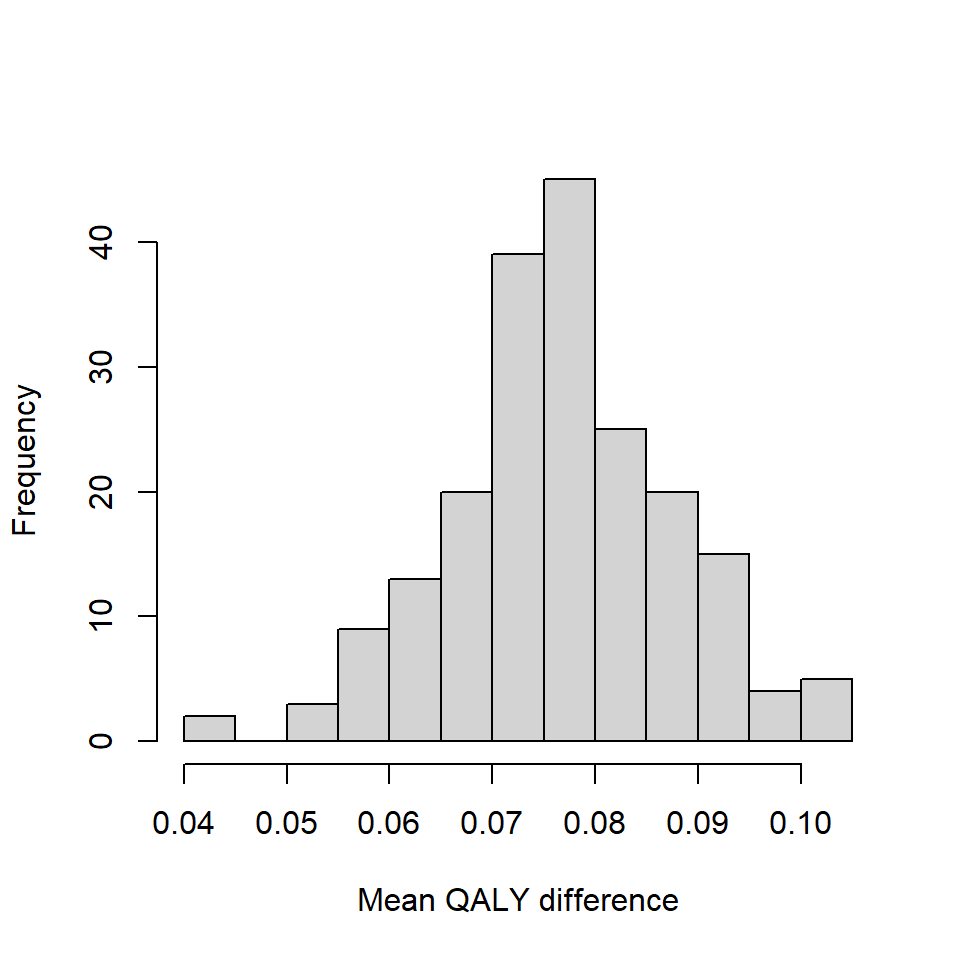
We can access the bootstrapped estimates for a given quantity, eg mean QALY and TC difference between treatment groups (New vs Old), by typing boot_res$QALY_boot$Delta_e and boot_res$QALY_boot$Delta_c, respectively. Once extracted, we can then inspect the distribution of \(\Delta_e\), for example, with an histogram.

In a similar way, the function also produces bootstrapped estimates for the mean QALY values in the comparator (Old) and reference (New) arm by typing boot_res$QALY_boot$mu_e_ctr and boot_res$QALY_boot$mu_e_int, which were derived at each bootstrap iteration using the same approach as in Section 1. Similar results with respect to the TC parameters can be obtained using the corresponding list names Delta_c,mu_c_ctr and mu_c_int.

Important Disclaimer. The above bootstrap function is quite flexible in that it allows to derive bootstrapped estimates for different CE quantities. However, it should NOT be implemented blindly. For example, when computing these quantities, it assumes that the treatment indicator is always placed as the first independent variable in both QALY and TC regression model formulae. If this is not true, then the estimates produced will be incorrect since they will correspond to the coefficients of some other independent variable! The position of the treatment indicator may be changed through a specific (optional) argument called trt_pos, by default set to \(2\) (since position \(1\) corresponds to the intercept in both models). In addition, mean outcome values for each treatment group are obtained as linear combination of the QALY/TC regression parameters in combination with specific covariate profiles (ie one for the comparator and one for the reference intervention). These profiles are computed under the assumption that, except the treatment indicator, all other independent variables should be set at their mean value. This is generally ok when interest is in the average estimates but makes little sense when interest is instead in retrieving estimates for specific covariate profiles. A typical example of this would be when a categorical or factor covariate (eg gender) is included in the models and that estimates for mean QALY/TC values should be produced for a given value for that variable (eg only for males). In this latter case, estimates produced by the default settings of the function will be incorrect since they are evaluated at the mean values for all covariates (except the treatment indicator). The function is provided with (optional) arguments called profile_QALY and profile_TC which allow the user to specify a custom covariate profile for each regression but, unless the user is familiar with how to correctly specify these profiles, care should be used in the interpretation of the generated estimates. All this to say, be careful about blindly using non-standard functions as, if you do not know how they work or how to interpret the output they produce, you may run the risk of generating completely nonsensical results!.

The entire bootstrap distribution of mean QALY/TC difference and/or those for the mean outcomes in each treatment group obtained through the function boot_ec may be used to generate standard CEA graphs such as the CE plane (Black 1990) and CE acceptability curve (Fenwick, Claxton, and Sculpher 2001). However, for the purpose of summarising uncertainty about the derived quantities, standard statistical measures such as confidence intervals should also be produced. Alternative ways to compute CIs based on bootstrapped estimates for a given quantity have been developed and compared, including in the context of CEA (Briggs, Wonderling, and Mooney 1997; Briggs, Mooney, and Wonderling 1999). Although initial methods focussed on the computation of CIs for Incremental Cost-Effectiveness Ratio (ICER), its ratio nature makes it quite difficult to provide sensible interpretations to confidence bounds in many scenarios (Glick et al. 2014). As a result, interest has been shifted towards the quantification of uncertainty via CIs for alternative quantities, such as the Net Monetary Benefit (NMB) which is a linear function of the mean differences in QALYs and TCs (Stinnett and Mullahy 1998).

The following (folded) code part shows how to obtain confidence intervals for any of the quantity derived from the boot_ec function using two popular approaches in the CEA literature: the empirical percentile (perc) method and the bias-corrected and accelerated (BCa) method. Although other approaches exist to derive confidence intervals for bootstrapped estimates, and a clear “best” approach in all possible scenarios has not been identified, these two approaches are by far those most commonly implemented in trial-based CEAs. In general, the perc approach is very easy to implement but has well known limitations, especially in small samples, in that it produces intervals that tend to be too narrow. The BCa approach, conversely, is generally regarded as a more robust version for computing intervals as it computes the CI bounds while introducing a bias and skewness correction term to improve the coverage performance in many scenarios (Briggs, Wonderling, and Mooney 1997). I have coded two functions, one called jk_ec, which is used to obtain jackknife estimates based on the original sample (needed to compute the BCa intervals), and another called boot_ci, which is the main function used to get the intervals. At the moment, both need to be loaded into the R workspace in order to compute the intervals and they also require as input the results generated by the previous function boot_ec.

#jackknife sampling function (used to compute BCa interval inside main boot_ci function)
jk_ec <- function(data,QALYreg,TCreg,trt_pos,profile_QALY_ctr,profile_QALY_int,
                   profile_TC_ctr,profile_TC_int,or_method){
  n <- dim(data)[1]
  #prepare objects to store results
  jk_delta_c_i <- jk_delta_e_i <- c()
  jk_mu0_c_i <- jk_mu0_e_i <- c()
  jk_mu1_c_i <- jk_mu1_e_i <- c()
  for(i in 1:n){
    #apply jackknife re-sampling
    data_i <- data[-i,]
    #obtain estimates of interest
    model_ec_i <- systemfit(list(QALYreg = QALYreg, TCreg = TCreg), 
                          method=or_method, data=data_i)
    jk_delta_e_i[i] <- summary(model_ec_i$eq[[1]])$coefficients[trt_pos,"Estimate"]
    jk_delta_c_i[i] <- summary(model_ec_i$eq[[2]])$coefficients[trt_pos,"Estimate"]
    jk_mu0_e_i[i] <- as.numeric(t(profile_QALY_ctr) %*% summary(model_ec_i$eq[[1]])$coefficients[,"Estimate"])
    jk_mu1_e_i[i] <- as.numeric(t(profile_QALY_int) %*% summary(model_ec_i$eq[[1]])$coefficients[,"Estimate"])
    jk_mu0_c_i[i] <- as.numeric(t(profile_TC_ctr) %*% summary(model_ec_i$eq[[2]])$coefficients[,"Estimate"])
    jk_mu1_c_i[i] <- as.numeric(t(profile_TC_int) %*% summary(model_ec_i$eq[[2]])$coefficients[,"Estimate"])
  }
  jk_est_i <- cbind.data.frame(jk_delta_e_i,jk_delta_c_i,jk_mu0_e_i,jk_mu1_e_i,jk_mu0_c_i,jk_mu1_c_i)
  names(jk_est_i) <- c("jk_Delta_e","jk_Delta_c","jk_mu_e_ctr","jk_mu_e_int","jk_mu_c_ctr","jk_mu_c_int")
  return(jk_est_i)
}

boot_ci <- function(x, method = "perc", confidence = 0.95){
  #the following lines are needed to make sure proper inputs are given
  if(!inherits(x, c("bootCE","tsbootCE"))) {stop("Only objects of class 'bootCE' or can 'tsbootCE' be used")}
  if(!method %in% c("perc","BCa")){stop("please provide valid method name")}
  if(!is.numeric(confidence)){stop("please provide valid confidence level")}
  if(confidence<=0 | confidence>=1){stop("please provide valid confidence level")}
  #extract information from inputs
  B <- length(x$QALY_boot$Delta_e)
  mu_e_ctr <- x$QALY_boot$mu_e_ctr
  mu_e_int <- x$QALY_boot$mu_e_int
  Delta_e <- x$QALY_boot$Delta_e
  mu_c_ctr <- x$TC_boot$mu_c_ctr
  mu_c_int <- x$TC_boot$mu_c_int
  Delta_c <- x$TC_boot$Delta_c
  alpha <- 1 - confidence
  #compute CI bounds according to method chosen
  if(method == "perc"){
    ci_mu_e_ctr <- quantile(mu_e_ctr, probs = c(alpha/2,(1-alpha/2)))
    ci_mu_e_int <- quantile(mu_e_int, probs = c(alpha/2,(1-alpha/2)))
    ci_Delta_e <- quantile(Delta_e, probs = c(alpha/2,(1-alpha/2)))
    ci_mu_c_ctr <- quantile(mu_c_ctr, probs = c(alpha/2,(1-alpha/2)))
    ci_mu_c_int <- quantile(mu_c_int, probs = c(alpha/2,(1-alpha/2)))
    ci_Delta_c <- quantile(Delta_c, probs = c(alpha/2,(1-alpha/2)))
  }
  if(method == "BCa"){
    or_method <- x$inputs$method
    data <- x$inputs$data
    trt_pos <- x$inputs$trt_pos
    QALYreg <- x$inputs$QALYreg
    TCreg <- x$inputs$TCreg
    profile_QALY_ctr <- x$inputs$profile_QALY_ctr
    profile_QALY_int <- x$inputs$profile_QALY_int
    profile_TC_ctr <- x$inputs$profile_TC_ctr
    profile_TC_int <- x$inputs$profile_TC_int
    #obtain avg BCa estimates based on original sample
    model_ec <- systemfit(list(QALYreg = QALYreg, TCreg = TCreg), 
                          method=or_method, data=data)
    avg_BCa_Delta_e <- summary(model_ec$eq[[1]])$coefficients[trt_pos,"Estimate"]
    avg_BCa_Delta_c <- summary(model_ec$eq[[2]])$coefficients[trt_pos,"Estimate"]
    avg_BCa_mu_e_ctr <- as.numeric(t(profile_QALY_ctr) %*% summary(model_ec$eq[[1]])$coefficients[,"Estimate"])
    avg_BCa_mu_e_int <- as.numeric(t(profile_QALY_int) %*% summary(model_ec$eq[[1]])$coefficients[,"Estimate"])
    avg_BCa_mu_c_ctr <- as.numeric(t(profile_TC_ctr) %*% summary(model_ec$eq[[2]])$coefficients[,"Estimate"])
    avg_BCa_mu_c_int <- as.numeric(t(profile_TC_int) %*% summary(model_ec$eq[[2]])$coefficients[,"Estimate"])
    #compute proportion of samples below avg estimates
    plower_Delta_e <- length(Delta_e[Delta_e<avg_BCa_Delta_e])/B
    plower_Delta_c <- length(Delta_c[Delta_c<avg_BCa_Delta_c])/B
    plower_mu_e_ctr <- length(mu_e_ctr[mu_e_ctr<avg_BCa_mu_e_ctr])/B
    plower_mu_e_int <- length(mu_e_int[mu_e_int<avg_BCa_mu_e_int])/B
    plower_mu_c_ctr <- length(mu_c_ctr[mu_c_ctr<avg_BCa_mu_c_ctr])/B
    plower_mu_c_int <- length(mu_c_int[mu_c_int<avg_BCa_mu_c_int])/B
    #compute bias-correction term
    z0_Delta_e <- qnorm(plower_Delta_e, mean = 0, sd = 1, lower.tail = TRUE)
    z0_Delta_c <- qnorm(plower_Delta_c, mean = 0, sd = 1, lower.tail = TRUE)
    z0_mu_e_ctr <- qnorm(plower_mu_e_ctr, mean = 0, sd = 1, lower.tail = TRUE)
    z0_mu_e_int <- qnorm(plower_mu_e_int, mean = 0, sd = 1, lower.tail = TRUE)
    z0_mu_c_ctr <- qnorm(plower_mu_c_ctr, mean = 0, sd = 1, lower.tail = TRUE)
    z0_mu_c_int <- qnorm(plower_mu_c_int, mean = 0, sd = 1, lower.tail = TRUE)
    #apply jackknife sampling functions to get jeckknife estimates
    jk_res <- jk_ec(data = data, QALYreg=QALYreg,TCreg=TCreg,trt_pos=trt_pos,
                        profile_QALY_ctr=profile_QALY_ctr,profile_QALY_int=profile_QALY_int,
                        profile_TC_ctr=profile_TC_ctr,profile_TC_int=profile_TC_int,or_method=or_method)
    #compute avg of jk estimates
    jk_res_avg <- apply(jk_res, 2, mean, na.rm=T) 
    #compute skewness correction term
    a_Delta_e <- sum((jk_res_avg["jk_Delta_e"] - jk_res[,"jk_Delta_e"])^3) / (6*(sum((jk_res_avg["jk_Delta_e"] - jk_res[,"jk_Delta_e"])^2))^(3/2))
    a_Delta_c <- sum((jk_res_avg["jk_Delta_c"] - jk_res[,"jk_Delta_c"])^3) / (6*(sum((jk_res_avg["jk_Delta_c"] - jk_res[,"jk_Delta_c"])^2))^(3/2))
    a_mu_e_ctr <- sum((jk_res_avg["jk_mu_e_ctr"] - jk_res[,"jk_mu_e_ctr"])^3) / (6*(sum((jk_res_avg["jk_mu_e_ctr"] - jk_res[,"jk_mu_e_ctr"])^2))^(3/2))
    a_mu_e_int <- sum((jk_res_avg["jk_mu_e_int"] - jk_res[,"jk_mu_e_int"])^3) / (6*(sum((jk_res_avg["jk_mu_e_int"] - jk_res[,"jk_mu_e_int"])^2))^(3/2))
    a_mu_c_ctr <- sum((jk_res_avg["jk_mu_c_ctr"] - jk_res[,"jk_mu_c_ctr"])^3) / (6*(sum((jk_res_avg["jk_mu_c_ctr"] - jk_res[,"jk_mu_c_ctr"])^2))^(3/2))
    a_mu_c_int <- sum((jk_res_avg["jk_mu_c_int"] - jk_res[,"jk_mu_c_int"])^3) / (6*(sum((jk_res_avg["jk_mu_c_int"] - jk_res[,"jk_mu_c_int"])^2))^(3/2))    
    #compute adjusted probs for getting desired confidence level
    z_alpha1 <- qnorm(alpha/2, mean = 0, sd = 1, lower.tail = TRUE)
    z_alpha2 <- qnorm(1-alpha/2, mean = 0, sd = 1, lower.tail = TRUE)
    ci_l_Delta_e <- pnorm(z0_Delta_e + ((z0_Delta_e+z_alpha1)/(1-a_Delta_e*(z0_Delta_e+z_alpha1))))
    ci_u_Delta_e <- pnorm(z0_Delta_e + ((z0_Delta_e+z_alpha2)/(1-a_Delta_e*(z0_Delta_e+z_alpha2))))
    ci_l_Delta_c <- pnorm(z0_Delta_c + ((z0_Delta_c+z_alpha1)/(1-a_Delta_c*(z0_Delta_c+z_alpha1))))
    ci_u_Delta_c <- pnorm(z0_Delta_c + ((z0_Delta_c+z_alpha2)/(1-a_Delta_c*(z0_Delta_c+z_alpha2))))
    ci_l_mu_e_ctr <- pnorm(z0_mu_e_ctr + ((z0_mu_e_ctr+z_alpha1)/(1-a_mu_e_ctr*(z0_mu_e_ctr+z_alpha1))))
    ci_u_mu_e_ctr <- pnorm(z0_mu_e_ctr + ((z0_mu_e_ctr+z_alpha2)/(1-a_mu_e_ctr*(z0_mu_e_ctr+z_alpha2))))
    ci_l_mu_e_int <- pnorm(z0_mu_e_int + ((z0_mu_e_int+z_alpha1)/(1-a_mu_e_int*(z0_mu_e_int+z_alpha1))))
    ci_u_mu_e_int <- pnorm(z0_mu_e_int + ((z0_mu_e_int+z_alpha2)/(1-a_mu_e_int*(z0_mu_e_int+z_alpha2))))
    ci_l_mu_c_ctr <- pnorm(z0_mu_c_ctr + ((z0_mu_c_ctr+z_alpha1)/(1-a_mu_c_ctr*(z0_mu_c_ctr+z_alpha1))))
    ci_u_mu_c_ctr <- pnorm(z0_mu_c_ctr + ((z0_mu_c_ctr+z_alpha2)/(1-a_mu_c_ctr*(z0_mu_c_ctr+z_alpha2))))
    ci_l_mu_c_int <- pnorm(z0_mu_c_int + ((z0_mu_c_int+z_alpha1)/(1-a_mu_c_int*(z0_mu_c_int+z_alpha1))))
    ci_u_mu_c_int <- pnorm(z0_mu_c_int + ((z0_mu_c_int+z_alpha2)/(1-a_mu_c_int*(z0_mu_c_int+z_alpha2))))
    #obtain quantiles on original scale
    ci_mu_e_ctr <- quantile(mu_e_ctr, probs = c(ci_l_mu_e_ctr,ci_u_mu_e_ctr))
    ci_mu_e_int <- quantile(mu_e_int, probs = c(ci_l_mu_e_int,ci_u_mu_e_int))
    ci_Delta_e <- quantile(Delta_e, probs = c(ci_l_Delta_e,ci_u_Delta_e))
    ci_mu_c_ctr <- quantile(mu_c_ctr, probs = c(ci_l_mu_c_ctr,ci_u_mu_c_ctr))
    ci_mu_c_int <- quantile(mu_c_int, probs = c(ci_l_mu_c_int,ci_u_mu_c_int))
    ci_Delta_c <- quantile(Delta_c, probs = c(ci_l_Delta_c,ci_u_Delta_c))
  }
  #organise and return results
  res_list <- list("Delta_e"=ci_Delta_e,"Delta_c"=ci_Delta_c,"mu_e_ctr"=ci_mu_e_ctr,"mu_e_int"=ci_mu_e_int,"mu_c_ctr"=ci_mu_c_ctr,"mu_c_int"=ci_mu_c_int)
  return(res_list)
}

As an example, we can now apply the newly created bootstrap function called boot_ci to our bootstrap results stored in the object boot_res to compute bootstrapped confidence intervals for all stored quantities using either the percentile or BCa approach (selected through the argument method).

#apply function to bootstrap results
boot_ci_bca <- boot_ci(x = boot_res, method = "BCa", confidence = 0.95)
boot_ci_bca

$Delta_e
 2.655003%  97.64746% 
0.05583106 0.09830066 

$Delta_c
1.886311% 96.72076% 
-15.25787  21.70418 

$mu_e_ctr
 3.48715% 98.23841% 
0.5612709 0.5915057 

$mu_e_int
2.478735% 97.47866% 
0.6361601 0.6636482 

$mu_c_ctr
2.907112% 97.85471% 
 283.1276  309.8906 

$mu_c_int
3.023147% 97.94824% 
 285.7260  313.8358 

The above code computes and displays \(95\%\) BCa intervals for each store quantity from the previous bootstrap function, namely the mean QALY and TC difference (\(\Delta_e, \Delta_c\)), and the mean QALY/TC in each treatment group (\(\mu_e,\mu_c\)), here referred to as “control” (ctr) and “intervetion” (int).

Summary

While SUR has been widely applied in trial-based CEA to account for the correlation between outcomes, mainly for its ease of implementation, its standalone implementation still has similar limitations to those of standard OLS approaches, eg reliance on Normality assumptions (see Section 1). For this reason it has been advocated the use of non-parametric bootstrapping as an alternative approach, which have been shown to produce adequate inferences while also retaining the correlation structure in the data through paired resampling methods. In addition, it is also possible to combine SUR and bootstrapping together within a single procedure, as also the code developed in this section showed.

However, due to its simulation-based nature, the performance of non-parametric bootstrapping in CEA for handling correlation has not been fully assessed and some areas of uncertainty remains. These include:

• Performance of bootstrapping with respect to proper joint models, which can formally take into account the correlation among multivariate outcomes. While joint models typically perform better for handling normally distributed outcomes, their relative performance with respect to non-parametric bootstrapping for non-normally distributed outcomes in small samples is still unclear.

• Alternative approaches for confidence intervals computation. Although, in the use of BCa methods is recommended, the relative performance of alternative approaches in general scenarios has not been fully assessed. In some case, eg small samples and high degree of skewness, some approaches to CI computation can lead to quite different results and are potentially biased/inefficient (Briggs, Wonderling, and Mooney 1997; Briggs, Mooney, and Wonderling 1999).

Despite the performance of bootstrapping not being fully assessed, its use in CEA is needed in that CE results need to be expressed in the form of “distributions” for the parameters of interest, eg mean QALY/TC incrementals and, within a frequentist framework, resampling methods allow to obtain empirical estimates of these distributions which can then be used to generate standard CEA output (eg CE plane). We note that, when a Bayesian framework is used instead, implementation of non-normal joint models becomes considerably easier and have been shown to perform quite well in the context of CEA (Nixon and Thompson 2005; Lambert et al. 2008; Conigliani and Tancredi 2009; Gabrio, Mason, and Baio 2019; Achana et al. 2021).

Skewness in CE outcomes

A general concern in trial-based CEA is the presence of high degrees of skewness in the outcome variables, especially costs. This is due to the specific nature of outcome data:

• Costs are bounded below at \(0\) and in many cases are characterised by empirical distributions that are highly skewed to the right (positively skewed), with many individuals associated with no or very low costs and a few individuals associated with very high costs.

• QoL utilities (used to construct QALYs) are bounded above at \(1\) and, especially in the context of non-life threatening interventions, are characterised by empirical distributions that are skewed to the left (negatively skewed), with many individuals associated with a perfect or high utility score (health state) and a few individuals associated with lower scores.

These features of CE data pose a threat to the validity of results derived from methods that rely on normality assumptions such as OLS and SUR models, or even parametric (eg Central Limit Theorem) and non-parametric (non-parametric tests or bootstrapping) methods that rely on asymptotic results, especially in the presence of high degree of skeweness and small samples (Thompson and Barber 2000; O’Hagan and Stevens 2003; Nixon, Wonderling, and Grieve 2010). The main problem is related to the definition of “too high” degree of skewness or “too small” sample size, on which a general consensus is lacking since performance of the methods can be highly affected by the specific combination of these two elements. In addition, options such as data transformation (eg take log) are not desirable since CE inference should be made on the arithmetic mean of the outcome variables on their original scale, which are usually not easily accessible when applying some transformation to the data (J. A. Barber and Thompson 2000).

To deal with skewness in small samples in CEA, the recommended approach in the literature consists in some form of Generalised Linear Model (GLM) regression framework (Thompson and Nixon 2005; J. Barber and Thompson 2004), which allow to choose alternative parametric distributional assumptions (eg Gamma) about the individual residuals to formally account for high levels of skewness. Although (non-parametric) bootstrapping is often advocated as a possible approach to handle skewness, its performance has been shown to be not optimal when facing high degrees of skewness in small samples (Nixon, Wonderling, and Grieve 2010). However, it is important to remember that, within a frequentist framework for CEA, use of bootstrapping is often required in order to generate approximate empirical distributions of the quantities of interest and use them to obtain standard CE output.

Data generation

In this section I will once more generate some artificial data that will be used to show how the desired methods can be implemented in R. The code used to generate these data is provided in the following (folded) code part and, if not of interest, you may skip it and jump to the actual implementation code in the next section.

#set parameter values for generating data
n_sam <- 20 #sample size
mu_u <- c(0.86,0.9)
sigma_u <- c(0.2,0.2)
tau_u <- (mu_u*(1-mu_u)/sigma_u^2-1)
shape1_u <- mu_u*tau_u
shape2_u <- (1-mu_u)*tau_u
mu_c <- c(100,125) 
sigma_c <- c(17,17)
shape_c <- mu_c^2/sigma_c^2
scale_c <- sigma_c^2/mu_c
#generaten QALY and TC data assuming Beta and Gamma distributions by arm
set.seed(2345)
sam0_u <- rbeta(n_sam/2,shape1 = shape1_u[1], shape2 = shape2_u[1])
sam1_u <- rbeta(n_sam/2,shape1 = shape1_u[2], shape2 = shape2_u[2])
sam0_c <- rgamma(n_sam/2, shape = shape_c[1], scale = scale_c[1])
sam1_c <- rgamma(n_sam/2, shape = shape_c[2], scale = scale_c[2])
#combine arm data and generate baseline u and c values
sam_u <- c(sam0_u,sam1_u)
base_u <- 0.75 + 0.5*sam_u + rnorm(n_sam, 0, 0.05) 
sam_c <- c(sam0_c,sam1_c)
base_c <- 50 + 0.01*sam_c + rnorm(n_sam, 0, 0.5) 
#create trt indicator
trt <- c(rep("old",n_sam/2),rep("new",n_sam/2))
#combine variables into a dataframe
dataset_sam_skew.df <- data.frame(sam_u,sam_c,base_u,base_c,trt)
names(dataset_sam_skew.df) <- c("QALY","TC","u","c","trt")
#randomly shuffle rows of the dataset
dataset_sam_skew.df <- dataset_sam_skew.df[sample(1:nrow(dataset_sam_skew.df)), ]
#define trt indicator as factor
dataset_sam_skew.df$trt <- factor(dataset_sam_skew.df$trt, levels = c("old","new"))

We can inspect the first few rows of the newly-generated data by typing

head(dataset_sam_skew.df, n=8)

        QALY        TC        u        c trt
16 0.9966611 118.19067 1.315029 51.47245 new
14 0.9970156 107.64264 1.253033 50.77574 new
12 0.9457835 132.33424 1.196667 51.32995 new
10 0.9496251  87.06468 1.294377 51.07543 old
3  0.9652897 102.36302 1.273476 51.03935 old
13 0.8985183 149.15977 1.259549 52.20984 new
4  0.6181245  86.65457 1.023924 50.95642 old
1  0.9931256 120.79056 1.229032 50.91415 old

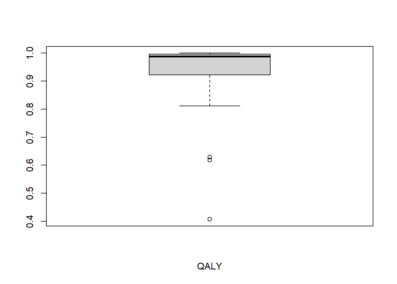
As an example, we can visually check the level of skewness for QALYs using boxplots, by typing

boxplot(dataset_sam_skew.df$QALY, ylab="",xlab="QALY")

Method application

Generalised Linear Models (GLM) share a similar regression framework to those of OLS and SUR (Section 1 and Section 2), where a given dependent variable, eg QALY or TC, is assumed to be a function of some independent variables through some regression coefficients \(\beta\) and some random error term \(\varepsilon_i\). A (simplified) representation of the GLM regression equations for the two CE outcomes may look something like:

\[ \begin{aligned} \text{E}[\text{QALY}_i] &= g_e(\beta_0 + \beta_1\times \text{arm}_i + \beta_2\times u_{i0})^{-1} \\ \text{E}[\text{TC}_i] &= g_c(\alpha_0 + \alpha_1\times \text{arm}_i + \alpha_2\times c_{i0})^{-1} \\ \end{aligned} \tag{5}\]

where \(\text{E}[\text{QALY}_i]\) and \(\text{E}[\text{TC}_i]\) denote the expected value of the two variables, expressed as a function of some regression coefficients and independent variables. Compared to standard regression, there are two main differences:

• The expected value is not a direct linear function of the parameters and variables, which are included linearly in the equation after some function \(g(\cdot)\) is applied. This is typical of GLM in that in many cases the range of the outcomes is bounded (above or below some values) and therefore a so-called link function \(g(\cdot)\) is used to allow a linear regression specification of the model on an unrestricted scale, which would otherwise be difficult to achieve. Estimates are then back-transformed on the original scale by applying the inverse function \(g(\cdot)^{-1}\). Examples of typical link functions include: log, logit, square root, and identity (ie no scaling). Their choice is mainly drive by the specific type of outcome variables and distributional assumptions made about the error term.

• The individual error term \(\varepsilon_i\) is not assumed to follow a normal distribution, but alternative parametric distributional forms are used, such as Beta, Gamma, Bernoulli, or Negative Binomial. The specific distributional choice is mainly driven again by the type of outcome variable which needs to be modelled.

In R, the following code may be used to fit GLMs as shown in Equation 5 assuming Beta-distributions for the QALY and Gamma distributions for the TC data, assuming a logit link function for the former and an identity link function for the latter. The code also shows how to summarise the generated output.

library(mfx) #load package to fit beta regression
#fit Beta regression to QALY assuming logit link
glm_e <- betareg(QALY ~ trt + u, data = dataset_sam_skew.df,  link = "logit")
#fit Gamma regression to TC assuming identity link
glm_c <- glm(TC ~ trt + c, data = dataset_sam_skew.df, family = Gamma(link = "identity"))
#summarise output
summary(glm_e)

Call:
betareg(formula = QALY ~ trt + u, data = dataset_sam_skew.df, link = "logit")

Quantile residuals:
    Min      1Q  Median      3Q     Max 
-2.0387 -0.4169  0.0253  0.5370  1.8036 

Coefficients (mean model with logit link):
            Estimate Std. Error z value            Pr(>|z|)    
(Intercept) -12.0426     1.6704  -7.209 0.00000000000056158 ***
trtnew        0.4970     0.4229   1.175                0.24    
u            12.2652     1.5441   7.943 0.00000000000000197 ***

Phi coefficients (precision model with identity link):
      Estimate Std. Error z value Pr(>|z|)   
(phi)   26.244      9.543    2.75  0.00596 **
---
Signif. codes:  0 '***' 0.001 '**' 0.01 '*' 0.05 '.' 0.1 ' ' 1 

Type of estimator: ML (maximum likelihood)
Log-likelihood: 54.13 on 4 Df
Pseudo R-squared: 0.4825
Number of iterations: 37 (BFGS) + 5 (Fisher scoring) 

summary(glm_c)

Call:
glm(formula = TC ~ trt + c, family = Gamma(link = "identity"), 
    data = dataset_sam_skew.df)

Coefficients:
            Estimate Std. Error t value Pr(>|t|)   
(Intercept) -463.632    284.001  -1.633  0.12096   
trtnew        25.654      6.729   3.812  0.00139 **
c             11.047      5.586   1.978  0.06442 . 
---
Signif. codes:  0 '***' 0.001 '**' 0.01 '*' 0.05 '.' 0.1 ' ' 1

(Dispersion parameter for Gamma family taken to be 0.01431784)

    Null deviance: 0.66693  on 19  degrees of freedom
Residual deviance: 0.24186  on 17  degrees of freedom
AIC: 165.32

Number of Fisher Scoring iterations: 5

Note that direct interpretation of the above model coefficients can be difficult due to the use of different link functions and non-normal distributional assumptions. However, we can use the convenient emmeans function from the package emmean to compute point and uncertainty estimates for mean QALY and TC variables on the original scale by treatment group (and the difference between groups using the contrast function) from the model output. The code part below shows how to do this.

#compute mean QALY and TC by arm on original scale
glm_e.em <- emmeans(glm_e, ~ trt)
glm_c.em <- emmeans(glm_c, ~ trt)

#print results for QALYs (example)
glm_e.em

 trt emmean     SE  df asymp.LCL asymp.UCL
 old  0.948 0.0144 Inf     0.920     0.976
 new  0.968 0.0108 Inf     0.947     0.989

Confidence level used: 0.95 

#specify and compute mean differences between groups (New - Old)
diff_NewvsOld <- list("New vs Old" = c(-1, 1))
glm_em_delta_e <- confint(contrast(glm_e.em, diff_NewvsOld))
glm_em_delta_c <- confint(contrast(glm_c.em, diff_NewvsOld))

#print results for QALYs difference (example)
glm_em_delta_e

 contrast   estimate     SE  df asymp.LCL asymp.UCL
 New vs Old   0.0196 0.0168 Inf   -0.0133    0.0525

Confidence level used: 0.95 

The following (folded) code part shows how to construct an R function which allows to implement a non-parametric bootstrap procedure for QALY and TC variables and derive bootstrapped estimates for marginal and incremental mean estimates by fitting a GLM to the outcomes for each bootstrapped sample.

#note that compared to the function developed before for OLS/SUR models, this one
#does not require to provide profiles for the computation of mean estimates but instead relies on the emmeans function to obtain these estimates without manual computation. Because of this the function is less flexible and can only evaluate mean estimates assuming a single profile for both QALY and TC models (the one used by emmeans to compute these quantities). However, the function needs the user to specify different distributions and link functions for the QALY and TC models. 
library(data.table)
library(rlang)
library(mfx) 
library(MASS)
library(bootstrap)
library(emmeans)
boot_ec_glm <- function(data, B, QALYreg, TCreg, QALY_dist, TC_dist, 
                        QALY_link, TC_link, trt_pos = 2){
  #the following lines are needed to make sure proper inputs are given
  if(!is.data.frame(data)){stop("data needs to be a data frame object")}
  if(!is.numeric(B)){stop("please provide number of bootstrap iterations")}
  if(B<=0 | !B%%1==0){stop("please provide number of bootstrap iterations")}
  if(!is_formula(QALYreg)){stop("please provide formula for QALY model")}
  if(!is_formula(TCreg)){stop("please provide formula for TC model")}
  if(!QALY_dist %in% c("Beta","Binomial","NegBinomial","Gamma","InvGaussian","Poisson","Gaussian")){stop("please provide valid distribution name")}
  if(!TC_dist %in% c("Beta","Binomial","NegBinomial","Gamma","InvGaussian","Poisson","Gaussian")){stop("please provide valid distribution name")}
  if(!QALY_link %in% c("logit","probit","cauchit", "cloglog", "identity", "log", "sqrt", "1/mu^2", "inverse")){stop("please provide valid link function name")}
  if(!TC_link %in% c("logit","probit","cauchit", "cloglog", "identity", "log", "sqrt", "1/mu^2", "inverse")){stop("please provide valid link function name")}
  if(!is.numeric(trt_pos) | length(trt_pos)!=1 | trt_pos<=0){stop("please provide valid trt indicator position in regressions")}
  n <- dim(data)[1] #original sample size
  #n covariates 
  nX_e <- dim(model.matrix(QALYreg, data))[2]
  nX_c <- dim(model.matrix(TCreg, data))[2]
  #extract name of trt indicator and outcomes from provided formula
  trt_name_e <- all.vars(QALYreg)[trt_pos]
  trt_name_c <- all.vars(TCreg)[trt_pos]
  if(trt_name_e != trt_name_c){stop("please provide same trt variable name and position in QALY and TC formuale")}
  QALY_name <- all.vars(QALYreg)[1]
  TC_name <- all.vars(TCreg)[1]
  #check if trt indicator is factor and store its levels
  if(is.factor(data[,trt_name_e])){
    trt_fact <- TRUE
    trt_lev <- levels(data[,trt_name_e])} else {
    trt_fact <- FALSE
    trt_lev <- unique(data[,trt_name_e])}
  if(length(trt_lev)!=2){stop("The function only allows comparison between two trt groups")}  
  #prepare empty objects to contain bootstrapped estimates
  data_ec_b_list <- list()
  coeff_e <- c()
  coeff_c <- c()
  em_e_ctr <- em_e_int <- c()
  em_c_ctr <- em_c_int <- c()
  dataset.dt <- data.table(data) #convert data into data.table object
  for(i in 1:B){
    #sample with replacement
    data_ec_b_list[[i]] <- dataset.dt[sample(.N, n, replace = T)]
    #select and fit GLM based on distribution and link function (QALY)
    if(QALY_dist=="Beta"){
      glm_e <- betareg(QALYreg, data = data_ec_b_list[[i]], link = QALY_link)}
    if(QALY_dist=="NegBinomial"){
      glm_e <- glm.nb(QALYreg, data = data_ec_b_list[[i]], link = QALY_link)}
    if(QALY_dist=="Binomial"){
      glm_e <- glm(QALYreg, data = data_ec_b_list[[i]], family = binomial(link = QALY_link))}
    if(QALY_dist=="Gamma"){
      glm_e <- glm(QALYreg, data = data_ec_b_list[[i]], family = Gamma(link = QALY_link))}
    if(QALY_dist=="InvGaussian"){
      glm_e <- glm(QALYreg, data = data_ec_b_list[[i]], family = inverse.gaussian(link = QALY_link))}
    if(QALY_dist=="Poisson"){
      glm_e <- glm(QALYreg, data = data_ec_b_list[[i]], family = poisson(link = QALY_link))} 
    if(QALY_dist=="Gaussian"){
      glm_e <- glm(QALYreg, data = data_ec_b_list[[i]], family = gaussian(link = QALY_link))}
    #select and fit GLM based on distribution and link function (TC)
    if(TC_dist=="Beta"){
      glm_c <- betareg(TCreg, data = data_ec_b_list[[i]], link = TC_link)}
    if(TC_dist=="NegBinomial"){
      glm_c <- glm.nb(TCreg, data = data_ec_b_list[[i]], link = TC_link)}
    if(TC_dist=="Binomial"){
      glm_c <- glm(TCreg, data = data_ec_b_list[[i]], family = binomial(link = TC_link))}
    if(TC_dist=="Gamma"){
      glm_c <- glm(TCreg, data = data_ec_b_list[[i]], family = Gamma(link = TC_link))}
    if(TC_dist=="InvGaussian"){
      glm_c <- glm(TCreg, data = data_ec_b_list[[i]], family = inverse.gaussian(link = TC_link))}
    if(TC_dist=="Poisson"){
      glm_c <- glm(TCreg, data = data_ec_b_list[[i]], family = poisson(link = TC_link))} 
    if(TC_dist=="Gaussian"){
      glm_c <- glm(TCreg, data = data_ec_b_list[[i]], family = gaussian(link = TC_link))}
    #use emmeans function to get mean outcomes for each arm
    glm_e.em <- emmeans(glm_e, trt_name_e, type = "response", data = data_ec_b_list[[i]])
    glm_c.em <- emmeans(glm_c, trt_name_c, type = "response", data = data_ec_b_list[[i]])
    em_e_ctr[i] <- summary(glm_e.em)[1,2]
    em_e_int[i] <- summary(glm_e.em)[2,2]
    em_c_ctr[i] <- summary(glm_c.em)[1,2]
    em_c_int[i] <- summary(glm_c.em)[2,2]
    #specify and compute mean differences between groups
    coeff_e[i] <- em_e_int[i] - em_e_ctr[i]
    coeff_c[i] <- em_c_int[i] - em_c_ctr[i]
  }
  #create list objects to store all results 
  res_e_b_list <-list("Delta_e"=coeff_e,"mu_e_ctr"=em_e_ctr,"mu_e_int"=em_e_int)
  res_c_b_list <-list("Delta_c"=coeff_c,"mu_c_ctr"=em_c_ctr,"mu_c_int"=em_c_int)
  input_list <- list("data"=data, "trt_pos"=trt_pos, "QALYreg"=QALYreg,
                     "TCreg"=TCreg,"QALY_link"=QALY_link,"QALY_dist"=QALY_dist,
                     "TC_dist"=TC_dist,"TC_link"=TC_link)
  #compute overall list and return it as output from the function
  res_ec_b_list <- list("QALY_boot"=res_e_b_list,"TC_boot"=res_c_b_list,"inputs"=input_list)
  class(res_ec_b_list) <- "bootCE_glm"
  return(res_ec_b_list)
}

We can now apply the newly created bootstrap function called boot_ec_glm to our generated dataset to obtain \(B=200\) bootstrapped estimates for the parameters of interest, which are here stored in a list object called boot_res_glm.

#set rng for reproducibility
set.seed(2345)
#apply function to dataset
boot_res_glm <- boot_ec_glm(data = dataset, QALYreg = QALY ~ trt + u,
                    TCreg = TC ~ trt + c, QALY_dist = "Beta", TC_dist = "Gamma",
                    QALY_link = "logit", TC_link = "inverse", B=200)

Note that, depending on the selected distribution and link function, GLMs may encounter problems in estimation and sometimes may not be even fit to some specific data. For example, if QALYs contain some negative values (which is theoretically possible), then Beta distributions will never be able to fit since these are defined on the interval \((0,1)\). These problems are also more likely to occur when implementing GLMs within a bootstrap procedure, since the resampling done at each iteration may lead to some data structures that do not fit well the assumed distributions.

Similarly to what done in Section 2, the following (folded) code part shows how to modify the function for generating bootstrap confidence intervals to allow the use of GLM results (produced through the function boot_ec_glm) instead of those from OLS and SUR models.

#jackknife sampling function (used to compute BCa interval inside main boot_ci function)
jk_ec_glm <- function(data,QALYreg,TCreg,trt_pos,QALY_dist,TC_dist,
                   QALY_link,TC_link){
  n <- dim(data)[1]
  #extract name of trt indicator from provided formula
  trt_name_e <- all.vars(QALYreg)[trt_pos]
  trt_name_c <- all.vars(TCreg)[trt_pos]
  #prepare objects to store results
  jk_delta_c_i <- jk_delta_e_i <- c()
  jk_mu0_c_i <- jk_mu0_e_i <- c()
  jk_mu1_c_i <- jk_mu1_e_i <- c()
  for(i in 1:n){
    #apply jackknife re-sampling
    data_i <- data[-i,]
    #obtain estimates of interest
    if(QALY_dist=="Beta"){
      glm_e <- betareg(QALYreg, data = data_i, link = QALY_link)}
    if(QALY_dist=="NegBinomial"){
      glm_e <- glm.nb(QALYreg, data = data_i, link = QALY_link)}
    if(QALY_dist=="Binomial"){
      glm_e <- glm(QALYreg, data = data_i, family = binomial(link = QALY_link))}
    if(QALY_dist=="Gamma"){
      glm_e <- glm(QALYreg, data = data_i, family = Gamma(link = QALY_link))}
    if(QALY_dist=="InvGaussian"){
      glm_e <- glm(QALYreg, data = data_i, family = inverse.gaussian(link = QALY_link))}
    if(QALY_dist=="Poisson"){
      glm_e <- glm(QALYreg, data = data_i, family = poisson(link = QALY_link))} 
    if(QALY_dist=="Gaussian"){
      glm_e <- glm(QALYreg, data = data_i, family = gaussian(link = QALY_link))}
    #select and fit GLM based on distribution and link function (TC)
    if(TC_dist=="Beta"){
      glm_c <- betareg(TCreg, data = data_i, link = TC_link)}
    if(TC_dist=="NegBinomial"){
      glm_c <- glm.nb(TCreg, data = data_i, link = TC_link)}
    if(TC_dist=="Binomial"){
      glm_c <- glm(TCreg, data = data_i, family = binomial(link = TC_link))}
    if(TC_dist=="Gamma"){
      glm_c <- glm(TCreg, data = data_i, family = Gamma(link = TC_link))}
    if(TC_dist=="InvGaussian"){
      glm_c <- glm(TCreg, data = data_i, family = inverse.gaussian(link = TC_link))}
    if(TC_dist=="Poisson"){
      glm_c <- glm(TCreg, data = data_i, family = poisson(link = TC_link))} 
    if(TC_dist=="Gaussian"){
      glm_c <- glm(TCreg, data = data_i, family = gaussian(link = TC_link))}    
    #use emmeans function to get mean outcomes for each arm
    glm_e.em <- emmeans(glm_e, trt_name_e, type = "response", data = data_i)
    glm_c.em <- emmeans(glm_c, trt_name_c, type = "response", data = data_i)
    jk_mu0_e_i[i] <- summary(glm_e.em)[1,2]
    jk_mu1_e_i[i] <- summary(glm_e.em)[2,2]
    jk_mu0_c_i[i] <- summary(glm_c.em)[1,2]
    jk_mu1_c_i[i] <- summary(glm_c.em)[2,2]
    #specify and compute mean differences between groups
    jk_delta_e_i[i] <- jk_mu1_e_i[i] - jk_mu0_e_i[i]
    jk_delta_c_i[i] <- jk_mu1_c_i[i] - jk_mu0_c_i[i]   
  }
  jk_est_i <- cbind.data.frame(jk_delta_e_i,jk_delta_c_i,jk_mu0_e_i,jk_mu1_e_i,jk_mu0_c_i,jk_mu1_c_i)
  names(jk_est_i) <- c("jk_Delta_e","jk_Delta_c","jk_mu_e_ctr","jk_mu_e_int","jk_mu_c_ctr","jk_mu_c_int")
  return(jk_est_i)
}

boot_ci_glm <- function(x, method = "perc", confidence = 0.95){
  #the following lines are needed to make sure proper inputs are given
  if(!inherits(x, c("bootCE_glm","tsbootCE_glm"))) {stop("Only objects of class 'bootCE_glm' or 'tsbootCE_glm' can be used")}
  if(!method %in% c("perc","BCa")){stop("please provide valid method name")}
  if(!is.numeric(confidence)){stop("please provide valid confidence level")}
  if(confidence<=0 | confidence>=1){stop("please provide valid confidence level")}
  #extract information from inputs
  B <- length(x$QALY_boot$Delta_e)
  mu_e_ctr <- x$QALY_boot$mu_e_ctr
  mu_e_int <- x$QALY_boot$mu_e_int
  Delta_e <- x$QALY_boot$Delta_e
  mu_c_ctr <- x$TC_boot$mu_c_ctr
  mu_c_int <- x$TC_boot$mu_c_int
  Delta_c <- x$TC_boot$Delta_c
  alpha <- 1 - confidence
  #compute CI bounds according to method chosen
  if(method == "perc"){
    ci_mu_e_ctr <- quantile(mu_e_ctr, probs = c(alpha/2,(1-alpha/2)))
    ci_mu_e_int <- quantile(mu_e_int, probs = c(alpha/2,(1-alpha/2)))
    ci_Delta_e <- quantile(Delta_e, probs = c(alpha/2,(1-alpha/2)))
    ci_mu_c_ctr <- quantile(mu_c_ctr, probs = c(alpha/2,(1-alpha/2)))
    ci_mu_c_int <- quantile(mu_c_int, probs = c(alpha/2,(1-alpha/2)))
    ci_Delta_c <- quantile(Delta_c, probs = c(alpha/2,(1-alpha/2)))
  }
  if(method == "BCa"){
    QALY_dist <- x$inputs$QALY_dist
    TC_dist <- x$inputs$TC_dist
    QALY_link <- x$inputs$QALY_link
    TC_link <- x$inputs$TC_link
    data <- x$inputs$data
    trt_pos <- x$inputs$trt_pos
    QALYreg <- x$inputs$QALYreg
    TCreg <- x$inputs$TCreg
    #obtain avg BCa estimates based on original sample
    if(QALY_dist=="Beta"){
      glm_e <- betareg(QALYreg, data = data, link = QALY_link)}
    if(QALY_dist=="NegBinomial"){
      glm_e <- glm.nb(QALYreg, data = data, link = QALY_link)}
    if(QALY_dist=="Binomial"){
      glm_e <- glm(QALYreg, data = data, family = binomial(link = QALY_link))}
    if(QALY_dist=="Gamma"){
      glm_e <- glm(QALYreg, data = data, family = Gamma(link = QALY_link))}
    if(QALY_dist=="InvGaussian"){
      glm_e <- glm(QALYreg, data = data, family = inverse.gaussian(link = QALY_link))}
    if(QALY_dist=="Poisson"){
      glm_e <- glm(QALYreg, data = data, family = poisson(link = QALY_link))} 
    if(QALY_dist=="Gaussian"){
      glm_e <- glm(QALYreg, data = data, family = gaussian(link = QALY_link))}
    #select and fit GLM based on distribution and link function (TC)
    if(TC_dist=="Beta"){
      glm_c <- betareg(TCreg, data = data, link = TC_link)}
    if(TC_dist=="NegBinomial"){
      glm_c <- glm.nb(TCreg, data = data, link = TC_link)}
    if(TC_dist=="Binomial"){
      glm_c <- glm(TCreg, data = data, family = binomial(link = TC_link))}
    if(TC_dist=="Gamma"){
      glm_c <- glm(TCreg, data = data, family = Gamma(link = TC_link))}
    if(TC_dist=="InvGaussian"){
      glm_c <- glm(TCreg, data = data, family = inverse.gaussian(link = TC_link))}
    if(TC_dist=="Poisson"){
      glm_c <- glm(TCreg, data = data, family = poisson(link = TC_link))} 
    if(TC_dist=="Gaussian"){
      glm_c <- glm(TCreg, data = data, family = gaussian(link = TC_link))}    
    #extract name of trt indicator from provided formula
    trt_name_e <- all.vars(QALYreg)[trt_pos]
    trt_name_c <- all.vars(TCreg)[trt_pos]
    #use emmeans function to get mean outcomes for each arm
    glm_e.em <- emmeans(glm_e, trt_name_e, type = "response", data = data)
    glm_c.em <- emmeans(glm_c, trt_name_c, type = "response", data = data)
    avg_BCa_mu_e_ctr <- summary(glm_e.em)[1,2]
    avg_BCa_mu_e_int <- summary(glm_e.em)[2,2]
    avg_BCa_mu_c_ctr <- summary(glm_c.em)[1,2]
    avg_BCa_mu_c_int <- summary(glm_c.em)[2,2]
    #specify and compute mean differences between groups
    avg_BCa_Delta_e <- avg_BCa_mu_e_int - avg_BCa_mu_e_ctr
    avg_BCa_Delta_c <- avg_BCa_mu_c_int - avg_BCa_mu_c_ctr    
    #compute proportion of samples below avg estimates
    plower_Delta_e <- length(Delta_e[Delta_e<avg_BCa_Delta_e])/B
    plower_Delta_c <- length(Delta_c[Delta_c<avg_BCa_Delta_c])/B
    plower_mu_e_ctr <- length(mu_e_ctr[mu_e_ctr<avg_BCa_mu_e_ctr])/B
    plower_mu_e_int <- length(mu_e_int[mu_e_int<avg_BCa_mu_e_int])/B
    plower_mu_c_ctr <- length(mu_c_ctr[mu_c_ctr<avg_BCa_mu_c_ctr])/B
    plower_mu_c_int <- length(mu_c_int[mu_c_int<avg_BCa_mu_c_int])/B
    #compute bias-correction term
    z0_Delta_e <- qnorm(plower_Delta_e, mean = 0, sd = 1, lower.tail = TRUE)
    z0_Delta_c <- qnorm(plower_Delta_c, mean = 0, sd = 1, lower.tail = TRUE)
    z0_mu_e_ctr <- qnorm(plower_mu_e_ctr, mean = 0, sd = 1, lower.tail = TRUE)
    z0_mu_e_int <- qnorm(plower_mu_e_int, mean = 0, sd = 1, lower.tail = TRUE)
    z0_mu_c_ctr <- qnorm(plower_mu_c_ctr, mean = 0, sd = 1, lower.tail = TRUE)
    z0_mu_c_int <- qnorm(plower_mu_c_int, mean = 0, sd = 1, lower.tail = TRUE)
    #apply jackknife sampling functions to get jeckknife estimates
    jk_res_glm <- jk_ec_glm(data = data, QALYreg=QALYreg,TCreg=TCreg,trt_pos=trt_pos,
                        QALY_dist=QALY_dist,TC_dist=TC_dist,
                        QALY_link=QALY_link,TC_link=TC_link)
    #compute avg of jk estimates
    jk_res_avg <- apply(jk_res_glm, 2, mean, na.rm = T) 
    #compute skewness correction term
    a_Delta_e <- sum((jk_res_avg["jk_Delta_e"] - jk_res_glm[,"jk_Delta_e"])^3) / (6*(sum((jk_res_avg["jk_Delta_e"] - jk_res_glm[,"jk_Delta_e"])^2))^(3/2))
    a_Delta_c <- sum((jk_res_avg["jk_Delta_c"] - jk_res_glm[,"jk_Delta_c"])^3) / (6*(sum((jk_res_avg["jk_Delta_c"] - jk_res_glm[,"jk_Delta_c"])^2))^(3/2))
    a_mu_e_ctr <- sum((jk_res_avg["jk_mu_e_ctr"] - jk_res_glm[,"jk_mu_e_ctr"])^3) / (6*(sum((jk_res_avg["jk_mu_e_ctr"] - jk_res_glm[,"jk_mu_e_ctr"])^2))^(3/2))
    a_mu_e_int <- sum((jk_res_avg["jk_mu_e_int"] - jk_res_glm[,"jk_mu_e_int"])^3) / (6*(sum((jk_res_avg["jk_mu_e_int"] - jk_res_glm[,"jk_mu_e_int"])^2))^(3/2))
    a_mu_c_ctr <- sum((jk_res_avg["jk_mu_c_ctr"] - jk_res_glm[,"jk_mu_c_ctr"])^3) / (6*(sum((jk_res_avg["jk_mu_c_ctr"] - jk_res_glm[,"jk_mu_c_ctr"])^2))^(3/2))
    a_mu_c_int <- sum((jk_res_avg["jk_mu_c_int"] - jk_res_glm[,"jk_mu_c_int"])^3) / (6*(sum((jk_res_avg["jk_mu_c_int"] - jk_res_glm[,"jk_mu_c_int"])^2))^(3/2))    
    #compute adjusted probs for getting desired confidence level
    z_alpha1 <- qnorm(alpha/2, mean = 0, sd = 1, lower.tail = TRUE)
    z_alpha2 <- qnorm(1-alpha/2, mean = 0, sd = 1, lower.tail = TRUE)
    ci_l_Delta_e <- pnorm(z0_Delta_e + ((z0_Delta_e+z_alpha1)/(1-a_Delta_e*(z0_Delta_e+z_alpha1))))
    ci_u_Delta_e <- pnorm(z0_Delta_e + ((z0_Delta_e+z_alpha2)/(1-a_Delta_e*(z0_Delta_e+z_alpha2))))
    ci_l_Delta_c <- pnorm(z0_Delta_c + ((z0_Delta_c+z_alpha1)/(1-a_Delta_c*(z0_Delta_c+z_alpha1))))
    ci_u_Delta_c <- pnorm(z0_Delta_c + ((z0_Delta_c+z_alpha2)/(1-a_Delta_c*(z0_Delta_c+z_alpha2))))
    ci_l_mu_e_ctr <- pnorm(z0_mu_e_ctr + ((z0_mu_e_ctr+z_alpha1)/(1-a_mu_e_ctr*(z0_mu_e_ctr+z_alpha1))))
    ci_u_mu_e_ctr <- pnorm(z0_mu_e_ctr + ((z0_mu_e_ctr+z_alpha2)/(1-a_mu_e_ctr*(z0_mu_e_ctr+z_alpha2))))
    ci_l_mu_e_int <- pnorm(z0_mu_e_int + ((z0_mu_e_int+z_alpha1)/(1-a_mu_e_int*(z0_mu_e_int+z_alpha1))))
    ci_u_mu_e_int <- pnorm(z0_mu_e_int + ((z0_mu_e_int+z_alpha2)/(1-a_mu_e_int*(z0_mu_e_int+z_alpha2))))
    ci_l_mu_c_ctr <- pnorm(z0_mu_c_ctr + ((z0_mu_c_ctr+z_alpha1)/(1-a_mu_c_ctr*(z0_mu_c_ctr+z_alpha1))))
    ci_u_mu_c_ctr <- pnorm(z0_mu_c_ctr + ((z0_mu_c_ctr+z_alpha2)/(1-a_mu_c_ctr*(z0_mu_c_ctr+z_alpha2))))
    ci_l_mu_c_int <- pnorm(z0_mu_c_int + ((z0_mu_c_int+z_alpha1)/(1-a_mu_c_int*(z0_mu_c_int+z_alpha1))))
    ci_u_mu_c_int <- pnorm(z0_mu_c_int + ((z0_mu_c_int+z_alpha2)/(1-a_mu_c_int*(z0_mu_c_int+z_alpha2))))
    #obtain quantiles on original scale
    ci_mu_e_ctr <- quantile(mu_e_ctr, probs = c(ci_l_mu_e_ctr,ci_u_mu_e_ctr))
    ci_mu_e_int <- quantile(mu_e_int, probs = c(ci_l_mu_e_int,ci_u_mu_e_int))
    ci_Delta_e <- quantile(Delta_e, probs = c(ci_l_Delta_e,ci_u_Delta_e))
    ci_mu_c_ctr <- quantile(mu_c_ctr, probs = c(ci_l_mu_c_ctr,ci_u_mu_c_ctr))
    ci_mu_c_int <- quantile(mu_c_int, probs = c(ci_l_mu_c_int,ci_u_mu_c_int))
    ci_Delta_c <- quantile(Delta_c, probs = c(ci_l_Delta_c,ci_u_Delta_c))
  }
  #organise and return results
  res_list <- list("Delta_e"=ci_Delta_e,"Delta_c"=ci_Delta_c,"mu_e_ctr"=ci_mu_e_ctr,"mu_e_int"=ci_mu_e_int,"mu_c_ctr"=ci_mu_c_ctr,"mu_c_int"=ci_mu_c_int)
  return(res_list)
}

#apply function to bootstrap results generated using the function boot_ec_glm to compute bootstrapped confidence intervals for all stored quantities using either the percentile or BCa approach (selected through the argument `method`).
boot_ci_glm_bca <- boot_ci_glm(x = boot_res_glm, method = "BCa", confidence = 0.95)

Summary

GLMs have been recommended as a valid approach to handle skewed data in CEA, although they are currently characterised by some drawbacks:

• Performance of the model may change substantially according to the specific parametric distributional assumptions made, with different distributions possibly leading to quite different results (Thompson and Nixon 2005). In theory, choice of an adequate distributional assumption allows to obtain more reliable estimates for the quantities of interest compared to methods that ignore skewness but assessment of a “good enough” fit of the selected distribution to the available data is difficult to establish.

• Choice of the link function may also have considerable impact on the fit of the model to the data- In general, link functions specified on the original scale are preferred to ease interpretation (eg identity link) but these often lead to instability of the estimates due to the non-symmetric nature of CE data, especially when multiple covariates are included in the models.

• Within a frequentist framework, implementation of joint GLMs is often difficult and impractical. This forces analysts to rely on fitting separate models to QALY and TC variables, therefore ignoring their possible correlation. This can be indirectly taken into account by embedding the models within a paired bootstrapping procedure, although its performance with respect to joint modelling has not been fully assessed.

More recently, methodological developments have been made in the context of Bayesian analysis of CE data, which allows a more flexible modelling framework compared to the standard frequentist approach. This lead to the development of so-called hurdle or two-part regression models in combination with non-normal distributional assumptions for CE outcomes to handle extremely skewed data even in small samples (Baio 2014; Gabrio, Mason, and Baio 2019). However, implementation of these methods within a frequentist framework can be very challenging, especially when these need to be combined with bootstrapping to generate empricial distributions for the estimates of interest required to perform the CE assessment.

Clustering of data

Some trials, for ethical or practical reasons, may randomise clusters rather than individual patients to each treatment arm. This is typically the case for cluster RCT, where the unit of randomisation becomes the treatment arm itself, ie individuals in a given cluster all receive the same treatment. When present, this design feature of the trial poses a threat to the validity of results derived from methods that ignore the clustering structure in the data, such as OLS, SUR or GLM approaches.

It has been shown that methods that ignore clustering (ie assume independence across all observations) will underestimate statistical uncertainty around parameter estimates, and may even result in biases and misleading conclusions (Gomes, Ng, et al. 2012). The problem is further exacerbated in the context of CEA where clustering needs to be addressed jointly with the other typical complexities affecting the data, such as the need to deal with baseline imbalances, correlation between the outcomes, and the level of skewness in both CE outcomes (Gomes, Grieve, et al. 2012).

Different approaches have been proposed in the literature to deal with clustering in CEA data and, among those assessed and compared, two main approaches have been suggested: Multilevel Models (MLM) and (non-parametric) Two-Stage Bootstrapping (TSB). The two approaches tackle the clustering problem from different perspectives but have been shown to perform good in general situations, although MLMs seem to have a generally better performance across a range of data structure scenarios (Gomes, Ng, et al. 2012).

Data generation

Let’s start by generating some artificial data that will be used to show how the desired methods can be implemented in R. The code used to generate these data is provided in the following (folded) code part and, if not of interest, you may skip it and jump to the actual implementation code in the next section.

#set parameter values for generating data
n <- 100 #sample size by cluster
J <- 26 #n of clusters
beta0_c <- 100
beta1_c <- 20
tau_c <- 10*2
trt_j <- c(rep(0,J/2),rep(1,J/2))
#simulate cluster-level means
set.seed(2345)
phi_cj <- rnorm(J,beta0_c+beta1_c*trt_j, tau_c) #cost cluster means
c_ij <- matrix(NA, nrow = n, ncol = J)
sigma_c <- 15*2
#simulate individual-level values
for(j in 1:J){
  c_ij[,j] <- rnorm(n,phi_cj[j],sigma_c) #cost data
}
beta0_e <- 0.5
beta1_e <- 0.1
tau_e <- 0.1*2
gamma <- tau_e/tau_c  #parameter capturing correlation between cluster QALY and cost means
#simulate cluster-level means
phi_ej <- rnorm(J,beta0_e+beta1_e+gamma*(phi_cj - (beta0_c+beta1_c*trt_j)), tau_e) #QALY cluster means
e_ij <- matrix(NA, nrow = n, ncol = J)
sigma_e <- 0.15*2
rho_ec <- 0.5
theta <- rho_ec*(sigma_e/sigma_c) #parameter capturing correlation between QALY and cost
#simulate individual-level values
for(j in 1:J){
  e_ij[,j] <- rnorm(n,phi_ej[j]+theta*(c_ij[,j]-phi_cj[j]),sigma_e)+rnorm(n,0,0.15) #QALY data
}
#compute ICC by outcome (cluster variance/total variance)
icc_c <- tau_c^2/(tau_c^2+sigma_c^2)
icc_e <- tau_e^2/(tau_e^2+sigma_e^2)
#generate dataset
cluster <- rep(1:J, each=n)
TC <- c(c_ij)
QALY <- c(e_ij)
trt <- ifelse(cluster<=13,"old","new")
id <- rep(1:n*J) #individual id number
data.clus.df <- data.frame(id, QALY,TC,trt,cluster)
data.clus.df$trt <- factor(data.clus.df$trt, levels = c("old","new"))
#randomly shuffle rows of the dataset
data.clus.df <- data.clus.df[sample(1:nrow(data.clus.df)), ]

We can inspect the first few rows of the newly-generated data by typing

head(data.clus.df, n=8)

       id       QALY       TC trt cluster
2228  728 1.23285753 108.9805 new      23
1351 1326 0.90037472 171.1320 new      14
374  1924 0.47126061 154.6768 old       4
1382 2132 0.67579513 135.2535 new      14
247  1222 0.10535644 109.3631 old       3
2324  624 0.04669856 104.4512 new      24
2128  728 1.22815612 104.2594 new      22
1656 1456 1.02208538 191.0768 new      17

and, as an example, we look at summary statistics for TC between two different clusters by typing

summary(data.clus.df$TC[data.clus.df$cluster==1])

   Min. 1st Qu.  Median    Mean 3rd Qu.    Max. 
  24.10   54.12   74.48   76.33   95.71  139.58 

summary(data.clus.df$TC[data.clus.df$cluster==15])

   Min. 1st Qu.  Median    Mean 3rd Qu.    Max. 
  63.24  105.11  128.03  125.58  143.45  190.73 

We can see that summary statistics can be quite different between clusters, therefore suggesting the violation of the independence assumption typical of standard statistical methods, such as OLS. We can also compute the Intraclass Correlation Coefficients (ICC) for the QALY (0.308) and TC (0.308) variables, which give an indication of the proportion of total variability in each outcome that is due to variability between clusters.

Method application

The general idea underlying MLM is to extend the standard OLS/SUR regression framework by adding some cluster-specific random terms to capture differences between cluster outcome means from the overall means computed across clusters. The regression model for the two CE outcomes can be expressed as:

\[ \begin{aligned} \text{QALY}_{ij} &= \beta_0 + \beta_1\times \text{arm}_j + u_{je} + \varepsilon_{ije} \\ \text{TC}_{ij} &= \alpha_0 + \alpha_1\times \text{arm}_j + u_{jc} + \varepsilon_{ijc} \\ \end{aligned} \tag{6}\]

where \(u_{je}\) and \(u_{jc}\) denote the random terms that are specific to cluster \(j\). Similarly to what discussed for SUR models (Equation 4), these error terms can be assumed to follow a joint normal distribution

\[ \begin{aligned} \begin{pmatrix} u_{je}\\ u_{jc}\\ \end{pmatrix} &\sim \text{Normal} \begin{bmatrix} \begin{pmatrix} 0\\ 0 \end{pmatrix}\!\!,& \begin{pmatrix} \tau^2_e & \psi\tau_e\tau_c\\ \psi\tau_c\tau_e & \tau^2_c \end{pmatrix} \end{bmatrix} \end{aligned} \]

where the parameter \(\psi\) allows to link the two random terms to capture possible correlation between cluster QALY and TC means, although it is often assumed \(0\) to ease implementation of the models.

In R, the following code may be used to fit separate MLM equations as shown in Equation 6 to the generated data and summarise the output:

library(lme4) #load package to fit MLM
library(nlme) #load package to fit MLM
#fit MLM to QALY regression
mlm_e <- lme(QALY ~ trt, random = ~1|cluster, data = data.clus.df)
summary(mlm_e) #summarise output

Linear mixed-effects model fit by REML
  Data: data.clus.df 
       AIC      BIC    logLik
  2244.443 2267.893 -1118.222

Random effects:
 Formula: ~1 | cluster
        (Intercept)  Residual
StdDev:   0.2747145 0.3642086

Fixed effects:  QALY ~ trt 
                Value  Std.Error   DF  t-value p-value
(Intercept) 0.5955004 0.07685878 2574 7.747981  0.0000
trtnew      0.0256487 0.10869473   24 0.235970  0.8155
 Correlation: 
       (Intr)
trtnew -0.707

Standardized Within-Group Residuals:
        Min          Q1         Med          Q3         Max 
-3.45114121 -0.70888295 -0.01460118  0.66186518  4.39502802 

Number of Observations: 2600
Number of Groups: 26 

#fit MLM to QALY regression
mlm_c <- lme(TC ~ trt, random = ~1|cluster, data = data.clus.df)
summary(mlm_c) #summarise output

Linear mixed-effects model fit by REML
  Data: data.clus.df 
       AIC      BIC    logLik
  25064.68 25088.13 -12528.34

Random effects:
 Formula: ~1 | cluster
        (Intercept) Residual
StdDev:    19.13406 29.46526

Fixed effects:  TC ~ trt 
               Value Std.Error   DF   t-value p-value
(Intercept) 99.40969  5.369388 2574 18.514155  0.0000
trtnew      20.25840  7.593462   24  2.667874  0.0135
 Correlation: 
       (Intr)
trtnew -0.707

Standardized Within-Group Residuals:
        Min          Q1         Med          Q3         Max 
-3.77623879 -0.68339399 -0.01845129  0.67128677  3.20459691 

Number of Observations: 2600
Number of Groups: 26 

We can use the function emmean from the R package emmeans to easily compute the mean QALYs in each treatment group. For example, we can type the following

library(emmeans) #load library to obtain marginal means
mlm1em_e <- emmeans(mlm_e, ~ trt) #compute mean outcome by level of trt
mlm1em_e

 trt emmean     SE df lower.CL upper.CL
 old  0.596 0.0769 25    0.437    0.754
 new  0.621 0.0769 24    0.463    0.780

Degrees-of-freedom method: containment 
Confidence level used: 0.95 

to directly obtain estimates of the mean QALYs, their standard errors and \(95\%\) confidence intervals by treatment group. We can then use the function contrast to derive estimates of any linear combination of the quantities above. For example, we may obtain estimates for the mean QALY difference (New - Old) by typing

#take difference as - Old + New = New - Old
QALY_new_vs_old <- list("New vs Old" = c(-1, 1))
#compute linear combination
mlm1em_delta_e <- contrast(mlm1em_e, QALY_new_vs_old)
#obtain results in terms of confidence intervals
confint(mlm1em_delta_e, level = 0.95)

 contrast   estimate    SE df lower.CL upper.CL
 New vs Old   0.0256 0.109 24   -0.199     0.25

Degrees-of-freedom method: containment 
Confidence level used: 0.95 

Although I have not shown here an application of MLM for TC estimates, these can be easily obtained in a similar way to what shown for QALYs.

In the (folded) code part below, I additionally provide R functions to implement MLMs within a boostrap procedure to generate bootstrapped estimates of the parameters of interest and their associated confidence intervals.

library(data.table) #package to handle datasets more efficiently
library(bootstrap) #package to use bootstrap procedure 
library(rlang)
library(lme4)
library(nlme)
library(emmeans)
boot_ec_mlm <- function(data, B, QALYreg, TCreg, QALYrandom, TCrandom, trt_pos = 2){
  #the following lines are needed to make sure proper inputs are given
  if(!is.data.frame(data)){stop("data needs to be a data frame object")}
  if(!is.numeric(B)){stop("please provide number of bootstrap iterations")}
  if(B<=0 | !B%%1==0){stop("please provide number of bootstrap iterations")}
  if(!is_formula(QALYreg)){stop("please provide formula for QALY model")}
  if(!is_formula(TCreg)){stop("please provide formula for TC model")}
  if(!is_formula(QALYrandom)){stop("please provide formula for QALY random effects")}
  if(!is_formula(TCrandom)){stop("please provide formula for TC random effects")}
  if(!is.numeric(trt_pos) | length(trt_pos)!=1 | trt_pos<=0){stop("please provide valid trt indicator position in regressions")}
  n <- dim(data)[1] #original sample size
  #n covariates 
  nX_e <- dim(model.matrix(QALYreg, data))[2]
  nX_c <- dim(model.matrix(TCreg, data))[2]
  #extract name of trt indicator and outcomes from provided formula
  trt_name_e <- all.vars(QALYreg)[trt_pos]
  trt_name_c <- all.vars(TCreg)[trt_pos]
  if(trt_name_e != trt_name_c){stop("please provide same trt variable name and position in QALY and TC formuale")}
  QALY_name <- all.vars(QALYreg)[1]
  TC_name <- all.vars(TCreg)[1]
  #check if trt indicator is factor and store its levels
  if(is.factor(data[,trt_name_e])){
    trt_fact <- TRUE
    trt_lev <- levels(data[,trt_name_e])} else {
    trt_fact <- FALSE
    trt_lev <- unique(data[,trt_name_e])}
  if(length(trt_lev)!=2){stop("The function only allows comparison between two trt groups")}  
  #prepare empty objects to contain bootstrapped estimates
  data_ec_b_list <- list()
  coeff_e <- c()
  coeff_c <- c()
  em_e_ctr <- em_e_int <- c()
  em_c_ctr <- em_c_int <- c()
  dataset.dt <- data.table(data) #convert data into data.table object
  for(i in 1:B){
    #sample with replacement
    data_ec_b_list[[i]] <- dataset.dt[sample(.N, n, replace = T)]
    #fit models for QALY and TC
    mlm_e <- lme(QALYreg, random = QALYrandom, data = data_ec_b_list[[i]])
    mlm_c <- lme(TCreg, random = TCrandom, data = data_ec_b_list[[i]])
    #use emmeans function to get mean outcomes for each arm
    mlm_e.em <- emmeans(mlm_e, trt_name_e, type = "response", data = data_ec_b_list[[i]])
    mlm_c.em <- emmeans(mlm_c, trt_name_c, type = "response", data = data_ec_b_list[[i]])
    em_e_ctr[i] <- summary(mlm_e.em)[1,2]
    em_e_int[i] <- summary(mlm_e.em)[2,2]
    em_c_ctr[i] <- summary(mlm_c.em)[1,2]
    em_c_int[i] <- summary(mlm_c.em)[2,2]
    #specify and compute mean differences between groups
    coeff_e[i] <- em_e_int[i] - em_e_ctr[i]
    coeff_c[i] <- em_c_int[i] - em_c_ctr[i]
  }
  #create list objects to store all results 
  res_e_b_list <-list("Delta_e"=coeff_e,"mu_e_ctr"=em_e_ctr,"mu_e_int"=em_e_int)
  res_c_b_list <-list("Delta_c"=coeff_c,"mu_c_ctr"=em_c_ctr,"mu_c_int"=em_c_int)
  input_list <- list("data"=data, "trt_pos"=trt_pos, "QALYreg"=QALYreg,
                     "TCreg"=TCreg,"QALYrandom"=QALYrandom,"TCrandom"=TCrandom)
  #compute overall list and return it as output from the function
  res_ec_b_list <- list("QALY_boot"=res_e_b_list,"TC_boot"=res_c_b_list,"inputs"=input_list)
  class(res_ec_b_list) <- "bootCE_mlm"
  return(res_ec_b_list)
}

#apply function to obtain bootstrap estimates from MLM
#set rng for reproducibility
set.seed(2345)
#the function fit separate MLM to QALY and TC data using normal random effects term specified for the variables indicated in the arguments QALYrandom and TCrandom, which must be specified as formulae following the notation indicated for random effects terms in the function lme from the package nlme
boot_res_mlm <- boot_ec_mlm(data = data.clus.df, QALYreg = QALY ~ trt, 
                            QALYrandom = ~1|cluster, TCreg = TC ~ trt, 
                            TCrandom = ~1|cluster, B=200)


#jackknife sampling function (used to compute BCa interval inside main boot_ci function)
jk_ec_mlm <- function(data,QALYreg,TCreg,trt_pos,QALYrandom,TCrandom){
  n <- dim(data)[1]
  #extract name of trt indicator from provided formula
  trt_name_e <- all.vars(QALYreg)[trt_pos]
  trt_name_c <- all.vars(TCreg)[trt_pos]
  #prepare objects to store results
  jk_delta_c_i <- jk_delta_e_i <- c()
  jk_mu0_c_i <- jk_mu0_e_i <- c()
  jk_mu1_c_i <- jk_mu1_e_i <- c()
  for(i in 1:n){
    #apply jackknife re-sampling
    data_i <- data[-i,]
    #fit models
    mlm_e <- lme(QALYreg, random = QALYrandom, data = data_i)
    mlm_c <- lme(TCreg, random = TCrandom, data = data_i)
    #use emmeans function to get mean outcomes for each arm
    mlm_e.em <- emmeans(mlm_e, trt_name_e, type = "response", data = data_i)
    mlm_c.em <- emmeans(mlm_c, trt_name_c, type = "response", data = data_i)
    jk_mu0_e_i[i] <- summary(mlm_e.em)[1,2]
    jk_mu1_e_i[i] <- summary(mlm_e.em)[2,2]
    jk_mu0_c_i[i] <- summary(mlm_c.em)[1,2]
    jk_mu1_c_i[i] <- summary(mlm_c.em)[2,2]
    #specify and compute mean differences between groups
    jk_delta_e_i[i] <- jk_mu1_e_i[i] - jk_mu0_e_i[i]
    jk_delta_c_i[i] <- jk_mu1_c_i[i] - jk_mu0_c_i[i]    
  }
  jk_est_i <- cbind.data.frame(jk_delta_e_i,jk_delta_c_i,jk_mu0_e_i,jk_mu1_e_i,jk_mu0_c_i,jk_mu1_c_i)
  names(jk_est_i) <- c("jk_Delta_e","jk_Delta_c","jk_mu_e_ctr","jk_mu_e_int","jk_mu_c_ctr","jk_mu_c_int")
  return(jk_est_i)
}

boot_ci_mlm <- function(x, method = "perc", confidence = 0.95){
  #the following lines are needed to make sure proper inputs are given
  if(!inherits(x, c("bootCE_mlm"))) {stop("Only objects of class 'bootCE_mlm' can be used")}
  if(!method %in% c("perc","BCa")){stop("please provide valid method name")}
  if(!is.numeric(confidence)){stop("please provide valid confidence level")}
  if(confidence<=0 | confidence>=1){stop("please provide valid confidence level")}
  #extract information from inputs
  B <- length(x$QALY_boot$Delta_e)
  mu_e_ctr <- x$QALY_boot$mu_e_ctr
  mu_e_int <- x$QALY_boot$mu_e_int
  Delta_e <- x$QALY_boot$Delta_e
  mu_c_ctr <- x$TC_boot$mu_c_ctr
  mu_c_int <- x$TC_boot$mu_c_int
  Delta_c <- x$TC_boot$Delta_c
  alpha <- 1 - confidence
  #compute CI bounds according to method chosen
  if(method == "perc"){
    ci_mu_e_ctr <- quantile(mu_e_ctr, probs = c(alpha/2,(1-alpha/2)))
    ci_mu_e_int <- quantile(mu_e_int, probs = c(alpha/2,(1-alpha/2)))
    ci_Delta_e <- quantile(Delta_e, probs = c(alpha/2,(1-alpha/2)))
    ci_mu_c_ctr <- quantile(mu_c_ctr, probs = c(alpha/2,(1-alpha/2)))
    ci_mu_c_int <- quantile(mu_c_int, probs = c(alpha/2,(1-alpha/2)))
    ci_Delta_c <- quantile(Delta_c, probs = c(alpha/2,(1-alpha/2)))
  }
  if(method == "BCa"){
    data <- x$inputs$data
    trt_pos <- x$inputs$trt_pos
    QALYreg <- x$inputs$QALYreg
    TCreg <- x$inputs$TCreg
    QALYrandom <- x$inputs$QALYrandom
    TCrandom <- x$inputs$TCrandom
    #obtain avg BCa estimates based on original sample
    mlm_e <- lme(QALYreg, random = QALYrandom, data = data)
    mlm_c <- lme(TCreg, random = TCrandom, data = data)
    #extract name of trt indicator from provided formula
    trt_name_e <- all.vars(QALYreg)[trt_pos]
    trt_name_c <- all.vars(TCreg)[trt_pos]
    #use emmeans function to get mean outcomes for each arm
    mlm_e.em <- emmeans(mlm_e, trt_name_e, type = "response", data = data)
    mlm_c.em <- emmeans(mlm_c, trt_name_c, type = "response", data = data)
    avg_BCa_mu_e_ctr <- summary(mlm_e.em)[1,2]
    avg_BCa_mu_e_int <- summary(mlm_e.em)[2,2]
    avg_BCa_mu_c_ctr <- summary(mlm_c.em)[1,2]
    avg_BCa_mu_c_int <- summary(mlm_c.em)[2,2]
    #specify and compute mean differences between groups
    avg_BCa_Delta_e <- avg_BCa_mu_e_int - avg_BCa_mu_e_ctr
    avg_BCa_Delta_c <- avg_BCa_mu_c_int - avg_BCa_mu_c_ctr     
    #compute proportion of samples below avg estimates
    plower_Delta_e <- length(Delta_e[Delta_e<avg_BCa_Delta_e])/B
    plower_Delta_c <- length(Delta_c[Delta_c<avg_BCa_Delta_c])/B
    plower_mu_e_ctr <- length(mu_e_ctr[mu_e_ctr<avg_BCa_mu_e_ctr])/B
    plower_mu_e_int <- length(mu_e_int[mu_e_int<avg_BCa_mu_e_int])/B
    plower_mu_c_ctr <- length(mu_c_ctr[mu_c_ctr<avg_BCa_mu_c_ctr])/B
    plower_mu_c_int <- length(mu_c_int[mu_c_int<avg_BCa_mu_c_int])/B
    #compute bias-correction term
    z0_Delta_e <- qnorm(plower_Delta_e, mean = 0, sd = 1, lower.tail = TRUE)
    z0_Delta_c <- qnorm(plower_Delta_c, mean = 0, sd = 1, lower.tail = TRUE)
    z0_mu_e_ctr <- qnorm(plower_mu_e_ctr, mean = 0, sd = 1, lower.tail = TRUE)
    z0_mu_e_int <- qnorm(plower_mu_e_int, mean = 0, sd = 1, lower.tail = TRUE)
    z0_mu_c_ctr <- qnorm(plower_mu_c_ctr, mean = 0, sd = 1, lower.tail = TRUE)
    z0_mu_c_int <- qnorm(plower_mu_c_int, mean = 0, sd = 1, lower.tail = TRUE)
    #apply jackknife sampling functions to get jeckknife estimates
    jk_res_mlm <- jk_ec_mlm(data = data, QALYreg=QALYreg,TCreg=TCreg,trt_pos=trt_pos,
                        QALYrandom=QALYrandom,TCrandom=TCrandom)
    #compute avg of jk estimates
    jk_res_avg <- apply(jk_res_mlm, 2, mean, na.rm=T) 
    #compute skewness correction term
    a_Delta_e <- sum((jk_res_avg["jk_Delta_e"] - jk_res_mlm[,"jk_Delta_e"])^3) / (6*(sum((jk_res_avg["jk_Delta_e"] - jk_res_mlm[,"jk_Delta_e"])^2))^(3/2))
    a_Delta_c <- sum((jk_res_avg["jk_Delta_c"] - jk_res_mlm[,"jk_Delta_c"])^3) / (6*(sum((jk_res_avg["jk_Delta_c"] - jk_res_mlm[,"jk_Delta_c"])^2))^(3/2))
    a_mu_e_ctr <- sum((jk_res_avg["jk_mu_e_ctr"] - jk_res_mlm[,"jk_mu_e_ctr"])^3) / (6*(sum((jk_res_avg["jk_mu_e_ctr"] - jk_res_mlm[,"jk_mu_e_ctr"])^2))^(3/2))
    a_mu_e_int <- sum((jk_res_avg["jk_mu_e_int"] - jk_res_mlm[,"jk_mu_e_int"])^3) / (6*(sum((jk_res_avg["jk_mu_e_int"] - jk_res_mlm[,"jk_mu_e_int"])^2))^(3/2))
    a_mu_c_ctr <- sum((jk_res_avg["jk_mu_c_ctr"] - jk_res_mlm[,"jk_mu_c_ctr"])^3) / (6*(sum((jk_res_avg["jk_mu_c_ctr"] - jk_res_mlm[,"jk_mu_c_ctr"])^2))^(3/2))
    a_mu_c_int <- sum((jk_res_avg["jk_mu_c_int"] - jk_res_mlm[,"jk_mu_c_int"])^3) / (6*(sum((jk_res_avg["jk_mu_c_int"] - jk_res_mlm[,"jk_mu_c_int"])^2))^(3/2))    
    #compute adjusted probs for getting desired confidence level
    z_alpha1 <- qnorm(alpha/2, mean = 0, sd = 1, lower.tail = TRUE)
    z_alpha2 <- qnorm(1-alpha/2, mean = 0, sd = 1, lower.tail = TRUE)
    ci_l_Delta_e <- pnorm(z0_Delta_e + ((z0_Delta_e+z_alpha1)/(1-a_Delta_e*(z0_Delta_e+z_alpha1))))
    ci_u_Delta_e <- pnorm(z0_Delta_e + ((z0_Delta_e+z_alpha2)/(1-a_Delta_e*(z0_Delta_e+z_alpha2))))
    ci_l_Delta_c <- pnorm(z0_Delta_c + ((z0_Delta_c+z_alpha1)/(1-a_Delta_c*(z0_Delta_c+z_alpha1))))
    ci_u_Delta_c <- pnorm(z0_Delta_c + ((z0_Delta_c+z_alpha2)/(1-a_Delta_c*(z0_Delta_c+z_alpha2))))
    ci_l_mu_e_ctr <- pnorm(z0_mu_e_ctr + ((z0_mu_e_ctr+z_alpha1)/(1-a_mu_e_ctr*(z0_mu_e_ctr+z_alpha1))))
    ci_u_mu_e_ctr <- pnorm(z0_mu_e_ctr + ((z0_mu_e_ctr+z_alpha2)/(1-a_mu_e_ctr*(z0_mu_e_ctr+z_alpha2))))
    ci_l_mu_e_int <- pnorm(z0_mu_e_int + ((z0_mu_e_int+z_alpha1)/(1-a_mu_e_int*(z0_mu_e_int+z_alpha1))))
    ci_u_mu_e_int <- pnorm(z0_mu_e_int + ((z0_mu_e_int+z_alpha2)/(1-a_mu_e_int*(z0_mu_e_int+z_alpha2))))
    ci_l_mu_c_ctr <- pnorm(z0_mu_c_ctr + ((z0_mu_c_ctr+z_alpha1)/(1-a_mu_c_ctr*(z0_mu_c_ctr+z_alpha1))))
    ci_u_mu_c_ctr <- pnorm(z0_mu_c_ctr + ((z0_mu_c_ctr+z_alpha2)/(1-a_mu_c_ctr*(z0_mu_c_ctr+z_alpha2))))
    ci_l_mu_c_int <- pnorm(z0_mu_c_int + ((z0_mu_c_int+z_alpha1)/(1-a_mu_c_int*(z0_mu_c_int+z_alpha1))))
    ci_u_mu_c_int <- pnorm(z0_mu_c_int + ((z0_mu_c_int+z_alpha2)/(1-a_mu_c_int*(z0_mu_c_int+z_alpha2))))
    #obtain quantiles on original scale
    ci_mu_e_ctr <- quantile(mu_e_ctr, probs = c(ci_l_mu_e_ctr,ci_u_mu_e_ctr))
    ci_mu_e_int <- quantile(mu_e_int, probs = c(ci_l_mu_e_int,ci_u_mu_e_int))
    ci_Delta_e <- quantile(Delta_e, probs = c(ci_l_Delta_e,ci_u_Delta_e))
    ci_mu_c_ctr <- quantile(mu_c_ctr, probs = c(ci_l_mu_c_ctr,ci_u_mu_c_ctr))
    ci_mu_c_int <- quantile(mu_c_int, probs = c(ci_l_mu_c_int,ci_u_mu_c_int))
    ci_Delta_c <- quantile(Delta_c, probs = c(ci_l_Delta_c,ci_u_Delta_c))
  }
  #organise and return results
  res_list <- list("Delta_e"=ci_Delta_e,"Delta_c"=ci_Delta_c,"mu_e_ctr"=ci_mu_e_ctr,"mu_e_int"=ci_mu_e_int,"mu_c_ctr"=ci_mu_c_ctr,"mu_c_int"=ci_mu_c_int)
  return(res_list)
}

#apply function to MLM results
boot_ci_mlm_bca <- boot_ci_mlm(x = boot_res_mlm, method = "BCa", confidence = 0.95)

An alternative approach to handle clustering in CEA is to combine standard statistical methods that ignore clustering (eg OLS, SUR or GLM) with a modified version of non-parametric bootstrapping, which takes the name of Two-Stage Bootstrapping (TSB). The key change consists in the way the sampling with replacement is performed from the original sample so to take into account the two-level data structure represented by clusters and individuals within clusters at each bootstrap iteration (Gomes, Ng, et al. 2012). In short, the TSB procedure can be summarised in the following steps:

1. Generate a “bootstrap” sample by sampling with replacement clusters from the original dataset and then sample QALY and TC individual values together within each resampled cluster
2. Fit the desired model to the newly obtained bootstrap sample to derive bootstrap estimates for the quantities of interest (eg mean outcome differences), for example using OLS or SUR models (ie \(\hat{\beta}^b_1\) and \(\hat{\alpha}^b_1\))
3. Repeat step 1-2 for a large number of bootstrap iterations \(B\) (eg \(5000\)) and store the results to generate a set of \(B\) bootstrap estimates for \(b=1,\ldots,B\)
4. Use the stored sets of bootstrap estimates (ie \(\hat{\beta}^b_1\) and \(\hat{\alpha}^b_1\)) to empirically approximate the sampling distribution of the parameters of interest.
5. Use this distribution of estimates to quantify the level of uncertainty around the quantities of interest, eg in terms of confidence intervals.

A limitation of standard TSB is that, due to the two-stage sampling procedure, it is very likely that the level of uncertainty, and so the variance of the estimated quantities, is overestimated. Thus, some form of shrinkage correction should be implemented within the TSB procedure to correct for variance overestimation (Gomes, Ng, et al. 2012). When using this correction, the TSB procedure is modified by shrinking cluster means and estimating individual residuals from the cluster means before any sampling is performed. Next, resampling is first applied to the shrunk cluster means, and then to the individual residuals. Finally, the resampled cluster means and individual residuals are combined to obtain a complete bootstrap sample, for which steps 2-5 are then followed.

The following (folded) code part shows how to construct an R function which allows to implement a non-parametric TSB procedure with shrinkage correction for QALY and TC variables and derive bootstrapped estimates for marginal and incremental mean estimates by fitting a OLS or SUR model to each bootstrapped sample.

library(data.table) #package to handle datasets more efficiently
library(bootstrap) #package to use bootstrap procedure 
library(rlang)
tsboot_ec <- function(data, B, QALYreg, TCreg, method = "OLS", cluster, unbalclus="donner",
                    profile_QALY="default", profile_TC="default", trt_pos = 2){
  #the following lines are needed to make sure proper inputs are given
  if(!is.data.frame(data)){stop("data needs to be a data frame object")}
  if(!is.numeric(B)){stop("please provide number of bootstrap iterations")}
  if(B<=0 | !B%%1==0){stop("please provide number of bootstrap iterations")}
  if(!is_formula(QALYreg)){stop("please provide formula for QALY model")}
  if(!is_formula(TCreg)){stop("please provide formula for TC model")}
  if(!method %in% c("OLS","SUR")){stop("please provide valid method name")}
  if(!is.numeric(trt_pos) | length(trt_pos)!=1 | trt_pos<=0){stop("please provide valid trt indicator position in regressions")}
  if(!is.character(cluster)){stop("please provide valid cluster variable name")}
  if(!cluster %in% names(data)){stop("please provide valid cluster variable name")}
  if(!unbalclus %in% c("donner","median","mean")){stop("please provide valid method to compute avg cluster size when standardising")}
  #convert cluster as factor and then numeric 
  data[,cluster] <- as.numeric(as.factor(data[,cluster]))
  #check that cluster variable is integer 
  if(!all(data[,cluster] - floor(data[,cluster]) == 0)){stop("cluster values should be integers")}
  n_size <- dim(data)[1] #original sample size
  #n covariates 
  nX_e <- dim(model.matrix(QALYreg, data))[2]
  nX_c <- dim(model.matrix(TCreg, data))[2]
  #check that correct profile provided or set default
  if(profile_QALY != "default"){
    if(!is.vector(profile_QALY) | length(profile_QALY)!=nX_e){stop("provide valid profile for QALYreg")}}
  if(profile_TC != "default"){
    if(!is.vector(profile_TC) | length(profile_TC)!=nX_c){stop("provide valid profile for TCreg")}}
  #extract name of trt indicator and outcomes from provided formula
  trt_name_e <- all.vars(QALYreg)[trt_pos]
  trt_name_c <- all.vars(TCreg)[trt_pos]
  if(trt_name_e != trt_name_c){stop("please provide same trt variable name and position in QALY and TC formuale")}
  QALY_name <- all.vars(QALYreg)[1]
  TC_name <- all.vars(TCreg)[1]
  #check if trt indicator is factor and store its levels
  if(is.factor(data[,trt_name_e])){
    trt_fact <- TRUE
    trt_lev <- levels(data[,trt_name_e])} else {
    trt_fact <- FALSE
    trt_lev <- unique(data[,trt_name_e])}
  if(length(trt_lev)!=2){stop("The function only allows comparison between two trt groups")}
  #prepare empty objects to contain bootstrapped estimates
  coeff_e <- c()
  coeff_c <- c()
  em_e_ctr <- em_e_int <- c()
  em_c_ctr <- em_c_int <- c()
for(i in 1:B){
    count <- 0 #set count for while loop across strata
    n.strata <- length(unique(data[,trt_name_e]))
    shrunk.data <- c()
  while (count<n.strata){
    count <- count+1
    data1 <- data.frame(data[data[,trt_name_e]==unique(data[,trt_name_e])[count],])
    clus.size <- table(data1[,cluster])
    cost.x <- tapply(data1[,TC_name],data1[,cluster],mean) # calc cluster means
    qaly.x <- tapply(data1[,QALY_name],data1[,cluster],mean) # calc cluster means
    # STANDARDIZE Z: calc b for standardiwing z
    a <- length(unique(data1[,cluster]))
    if (var(clus.size)==0){
     b <- unique(clus.size)
   } else {
    if (unbalclus=="donner"){
     ifelse(warning,print("'average' clus size = Donner"),NA)
     n <- sum(clus.size)
     b <- (n-(sum(clus.size^2)/n))/(a-1)
    } else if (unbalclus=="median"){
     ifelse(warning,print("'average' clus size = median"),NA)
     b <- median(clus.size)
    } else if (unbalclus=="mean"){
     ifelse(warning,print("'average' clus size = mean"),NA)
     b <- mean(clus.size)
    } else {}
   } # End of 'else'
    # standardise z using cluster means (dfm = deviation from cluster mean)
    cost.dfm <- data1[,TC_name]-rep(cost.x,times=clus.size)
    qaly.dfm <- data1[,QALY_name]-rep(qaly.x,times=clus.size)
    cost.z <- (cost.dfm)/sqrt(1-1/b)
    qaly.z <- (qaly.dfm)/sqrt(1-1/b)
    # SHRINKAGE: calc c for shrinking x
    cost.ssw <- sum(cost.dfm^2)
    qaly.ssw <- sum(qaly.dfm^2)
    cost.ssb <- sum((cost.x-mean(cost.x))^2)
    qaly.ssb <- sum((qaly.x-mean(qaly.x))^2)
    cost.rhs <- a/(a-1) - cost.ssw/(b*(b-1)*cost.ssb)
    qaly.rhs <- a/(a-1) - qaly.ssw/(b*(b-1)*qaly.ssb)
    ifelse(cost.rhs<0, cost.c<-1, cost.c<-1-sqrt(cost.rhs))
    ifelse(qaly.rhs<0, qaly.c<-1, qaly.c<-1-sqrt(qaly.rhs))
    ## re-calc x
    cost.x <- cost.c*mean(data1[,TC_name]) + (1-cost.c)*cost.x
    qaly.x <- qaly.c*mean(data1[,QALY_name]) + (1-qaly.c)*qaly.x
    # TWO-STAGE SAMPLING & RE-CONSTRUCT OBS WITH SHRUNKEN MEANS AND STANDARDISED RESIDUALS
    # gen random clus (order) id with replacement
    sampled.x.cid <- sample(1:length(unique(data1[,cluster])),replace=T)
    sampled.z.iid <- sample(1:length(cost.z),sum(clus.size[sampled.x.cid]),replace=T) # chosen ind ids     for varying stratum sizes
    sampled.cost <- rep(cost.x[sampled.x.cid],times=clus.size[sampled.x.cid])+cost.z[sampled.z.iid]
    sampled.qaly <- rep(qaly.x[sampled.x.cid],times=clus.size[sampled.x.cid])+qaly.z[sampled.z.iid]
    # bind data from multiple strata together
    shrunk.data <- as.data.frame(rbind(shrunk.data,cbind(sampled.cost,sampled.qaly,
    rep(unique(data1[,cluster])[sampled.x.cid],times=clus.size[sampled.x.cid]),
    rep(unique(data[,trt_name_e])[count],times=sum(clus.size[sampled.x.cid])))))
  } # end of while
  #rename variables
  colnames(shrunk.data) <- c(TC_name,QALY_name,cluster,trt_name_e)
  #copy trt levels if factor
  if(is_true(trt_fact)){ 
    shrunk.data[,trt_name_e] <- factor(shrunk.data[,trt_name_e], levels=sort(unique(shrunk.data[,trt_name_e])), labels = trt_lev)}
    #create a dt object
    dataset_tsb.dt <- data.table(shrunk.data)
    #fit model
    model_ec <- systemfit(list(QALYreg = QALYreg, TCreg = TCreg), 
                          method=method, data=dataset_tsb.dt)
    #extract covariate values
    X_e <- model.matrix(model_ec$eq[[1]])
    X_c <- model.matrix(model_ec$eq[[2]])
    #define QALYreg profile
    if(profile_QALY == "default"){
     profile_b_QALY <- apply(X_e, 2, mean, na.rm=T)
    } else {profile_b_QALY <- profile_QALY}
    profile_b_QALY_ctr <- profile_b_QALY_int <- profile_b_QALY
    profile_b_QALY_ctr[trt_pos] <- 0 #set profile for comparator
    profile_b_QALY_int[trt_pos] <- 1 #set profile for reference
    #define TCreg profile
    if(profile_TC == "default"){
     profile_b_TC <- apply(X_c, 2, mean, na.rm=T)
    } else {profile_b_TC <- profile_TC}
    profile_b_TC_ctr <- profile_b_TC_int <- profile_b_TC
    profile_b_TC_ctr[trt_pos] <- 0 #set profile for comparator
    profile_b_TC_int[trt_pos] <- 1 #set profile for reference
    #extract coefficient estimates from each model
    coeff_e[i] <- summary(model_ec$eq[[1]])$coefficients[trt_pos,"Estimate"]
    coeff_c[i] <- summary(model_ec$eq[[2]])$coefficients[trt_pos,"Estimate"]
    #compute linear combination of parameters
    em_e_ctr[i] <- t(profile_b_QALY_ctr) %*% summary(model_ec$eq[[1]])$coefficients[,"Estimate"] 
    em_e_int[i] <- t(profile_b_QALY_int) %*% summary(model_ec$eq[[1]])$coefficients[,"Estimate"] 
    em_c_ctr[i] <- t(profile_b_TC_ctr) %*% summary(model_ec$eq[[2]])$coefficients[,"Estimate"] 
    em_c_int[i] <- t(profile_b_TC_int) %*% summary(model_ec$eq[[2]])$coefficients[,"Estimate"] 
  }
  #create list objects to store all results 
  res_e_tsb_list <-list("Delta_e"=coeff_e,"mu_e_ctr"=em_e_ctr,"mu_e_int"=em_e_int)
  res_c_tsb_list <-list("Delta_c"=coeff_c,"mu_c_ctr"=em_c_ctr,"mu_c_int"=em_c_int)
  input_list <- list("data"=data, "method"=method, "trt_pos"=trt_pos, "QALYreg"=QALYreg,
                     "TCreg"=TCreg,"profile_QALY_ctr"=profile_b_QALY_ctr,
                     "profile_QALY_int"=profile_b_QALY_int,"profile_TC_ctr"=profile_b_TC_ctr,
                     "profile_TC_int"=profile_b_TC_int, "cluster"=cluster, "unbalclus"=unbalclus)
  #compute overall list and return it as output from the function
  res_ec_tsb_list <- list("QALY_boot"=res_e_tsb_list,"TC_boot"=res_c_tsb_list,"inputs"=input_list)
  class(res_ec_tsb_list) <- "tsbootCE"
  return(res_ec_tsb_list)
}

We can now apply the newly created TSB function called tsboot_res to our generated dataset to obtain \(B=200\) bootstrapped estimates for the parameters of interest, which are here stored in a list object called tsboot_res.

#set rng for reproducibility
set.seed(2345)
#apply function to dataset
tsboot_res <- tsboot_ec(data = data.clus.df, QALYreg = QALY ~ trt, cluster = "cluster", TCreg = TC ~ trt, method = "OLS", B=200)

Next, we can use the functions jk_ec and boot_ci shown in Section 2 to compute bootstrapped confidence intervals. As an example, we can now apply the newly created bootstrap function called boot_ci to our bootstrap results stored in the object tsboot_res to compute bootstrapped confidence intervals for all stored quantities using either the BCa approach (selected through the argument method).

#apply function to TSB results
tsboot_ci_bca <- boot_ci(x = tsboot_res, method = "BCa", confidence = 0.95)
tsboot_ci_bca

$Delta_e
0.5842263%  91.91954% 
-0.1961036  0.1850060 

$Delta_c
0.8417625%  93.69878% 
  2.949009  32.641264 

$mu_e_ctr
5.173335% 98.90882% 
0.4810873 0.7642355 

$mu_e_int
1.631128% 96.27396% 
0.4918447 0.7677400 

$mu_c_ctr
8.490612% 99.46002% 
 92.51988 112.04817 

$mu_c_int
1.857534% 96.67969% 
 109.7356  130.1179 

For completeness, in the following (folded) code part, I also provide the same TSB functions but tailored to the specification of independent GLMs rather than OLS/SUR models only possible with tsboot_res.

#note that compared to the function developed before for OLS/SUR models, this one
#does not require to provide profiles for the computation of mean estimates but instead relies on the emmeans function to obtain these estimates without manual computation. Because of this the function is less flexible and can only evaluate mean estimates assuming a single profile for both QALY and TC models (the one used by emmeans to compute these quantities). However, the function needs the user to specify different distributions and link functions for the QALY and TC models. 
library(data.table)
library(rlang)
library(mfx) 
library(MASS)
library(bootstrap)
library(emmeans)
tsboot_ec_glm <- function(data, B, QALYreg, TCreg, QALY_dist, TC_dist, 
                        QALY_link, TC_link, cluster, unbalclus="donner", trt_pos = 2){
  #the following lines are needed to make sure proper inputs are given
  if(!is.data.frame(data)){stop("data needs to be a data frame object")}
  if(!is.numeric(B)){stop("please provide number of bootstrap iterations")}
  if(B<=0 | !B%%1==0){stop("please provide number of bootstrap iterations")}
  if(!is_formula(QALYreg)){stop("please provide formula for QALY model")}
  if(!is_formula(TCreg)){stop("please provide formula for TC model")}
  if(!QALY_dist %in% c("Beta","Binomial","NegBinomial","Gamma","InvGaussian","Poisson","Gaussian")){stop("please provide valid distribution name")}
  if(!TC_dist %in% c("Beta","Binomial","NegBinomial","Gamma","InvGaussian","Poisson","Gaussian")){stop("please provide valid distribution name")}
  if(!QALY_link %in% c("logit","probit","cauchit", "cloglog", "identity", "log", "sqrt", "1/mu^2", "inverse")){stop("please provide valid link function name")}
  if(!TC_link %in% c("logit","probit","cauchit", "cloglog", "identity", "log", "sqrt", "1/mu^2", "inverse")){stop("please provide valid link function name")}
  if(!is.numeric(trt_pos) | length(trt_pos)!=1 | trt_pos<=0){stop("please provide valid trt indicator position in regressions")}
  if(!is.character(cluster)){stop("please provide valid cluster variable name")}
  if(!cluster %in% names(data)){stop("please provide valid cluster variable name")}
  if(!unbalclus %in% c("donner","median","mean")){stop("please provide valid method to compute avg cluster size when standardising")}
  #convert cluster as factor and then numeric 
  data[,cluster] <- as.numeric(as.factor(data[,cluster]))
  #check that cluster variable is integer 
  if(!all(data[,cluster] - floor(data[,cluster]) == 0)){stop("cluster values should be integers")}
  n_size <- dim(data)[1] #original sample size
  #n covariates 
  nX_e <- dim(model.matrix(QALYreg, data))[2]
  nX_c <- dim(model.matrix(TCreg, data))[2]
  #extract name of trt indicator and outcomes from provided formula
  trt_name_e <- all.vars(QALYreg)[trt_pos]
  trt_name_c <- all.vars(TCreg)[trt_pos]
  if(trt_name_e != trt_name_c){stop("please provide same trt variable name and position in QALY and TC formuale")}
  QALY_name <- all.vars(QALYreg)[1]
  TC_name <- all.vars(TCreg)[1]
  #check if trt indicator is factor and store its levels
  if(is.factor(data[,trt_name_e])){
    trt_fact <- TRUE
    trt_lev <- levels(data[,trt_name_e])} else {
    trt_fact <- FALSE
    trt_lev <- unique(data[,trt_name_e])}
  if(length(trt_lev)!=2){stop("The function only allows comparison between two trt groups")}
  #prepare empty objects to contain bootstrapped estimates
  coeff_e <- c()
  coeff_c <- c()
  em_e_ctr <- em_e_int <- c()
  em_c_ctr <- em_c_int <- c()
for(i in 1:B){
    count <- 0 #set count for while loop across strata
    n.strata <- length(unique(data[,trt_name_e]))
    shrunk.data <- c()
  while (count<n.strata){
    count <- count+1
    data1 <- data.frame(data[data[,trt_name_e]==unique(data[,trt_name_e])[count],])
    clus.size <- table(data1[,cluster])
    cost.x <- tapply(data1[,TC_name],data1[,cluster],mean) # calc cluster means
    qaly.x <- tapply(data1[,QALY_name],data1[,cluster],mean) # calc cluster means
    # STANDARDIZE Z: calc b for standardiwing z
    a <- length(unique(data1[,cluster]))
    if (var(clus.size)==0){
     b <- unique(clus.size)
   } else {
    if (unbalclus=="donner"){
     ifelse(warning,print("'average' clus size = Donner"),NA)
     n <- sum(clus.size)
     b <- (n-(sum(clus.size^2)/n))/(a-1)
    } else if (unbalclus=="median"){
     ifelse(warning,print("'average' clus size = median"),NA)
     b <- median(clus.size)
    } else if (unbalclus=="mean"){
     ifelse(warning,print("'average' clus size = mean"),NA)
     b <- mean(clus.size)
    } else {}
   } # End of 'else'
    # standardise z using cluster means (dfm = deviation from cluster mean)
    cost.dfm <- data1[,TC_name]-rep(cost.x,times=clus.size)
    qaly.dfm <- data1[,QALY_name]-rep(qaly.x,times=clus.size)
    cost.z <- (cost.dfm)/sqrt(1-1/b)
    qaly.z <- (qaly.dfm)/sqrt(1-1/b)
    # SHRINKAGE: calc c for shrinking x
    cost.ssw <- sum(cost.dfm^2)
    qaly.ssw <- sum(qaly.dfm^2)
    cost.ssb <- sum((cost.x-mean(cost.x))^2)
    qaly.ssb <- sum((qaly.x-mean(qaly.x))^2)
    cost.rhs <- a/(a-1) - cost.ssw/(b*(b-1)*cost.ssb)
    qaly.rhs <- a/(a-1) - qaly.ssw/(b*(b-1)*qaly.ssb)
    ifelse(cost.rhs<0, cost.c<-1, cost.c<-1-sqrt(cost.rhs))
    ifelse(qaly.rhs<0, qaly.c<-1, qaly.c<-1-sqrt(qaly.rhs))
    ## re-calc x
    cost.x <- cost.c*mean(data1[,TC_name]) + (1-cost.c)*cost.x
    qaly.x <- qaly.c*mean(data1[,QALY_name]) + (1-qaly.c)*qaly.x
    # TWO-STAGE SAMPLING & RE-CONSTRUCT OBS WITH SHRUNKEN MEANS AND STANDARDISED RESIDUALS
    # gen random clus (order) id with replacement
    sampled.x.cid <- sample(1:length(unique(data1[,cluster])),replace=T)
    sampled.z.iid <- sample(1:length(cost.z),sum(clus.size[sampled.x.cid]),replace=T) # chosen ind ids     for varying stratum sizes
    sampled.cost <- rep(cost.x[sampled.x.cid],times=clus.size[sampled.x.cid])+cost.z[sampled.z.iid]
    sampled.qaly <- rep(qaly.x[sampled.x.cid],times=clus.size[sampled.x.cid])+qaly.z[sampled.z.iid]
    # bind data from multiple strata together
    shrunk.data <- as.data.frame(rbind(shrunk.data,cbind(sampled.cost,sampled.qaly,
    rep(unique(data1[,cluster])[sampled.x.cid],times=clus.size[sampled.x.cid]),
    rep(unique(data[,trt_name_e])[count],times=sum(clus.size[sampled.x.cid])))))
  } # end of while
  #rename variables
  colnames(shrunk.data) <- c(TC_name,QALY_name,cluster,trt_name_e)
  #copy trt levels if factor
  if(is_true(trt_fact)){ 
    shrunk.data[,trt_name_e] <- factor(shrunk.data[,trt_name_e], levels=sort(unique(shrunk.data[,trt_name_e])), labels = trt_lev)}
    #create a dt object
    dataset_tsb.dt <- data.table(shrunk.data)
    #select and fit GLM based on distribution and link function (QALY)
    if(QALY_dist=="Beta"){
      glm_e <- betareg(QALYreg, data = dataset_tsb.dt, link = QALY_link)}
    if(QALY_dist=="NegBinomial"){
      glm_e <- glm.nb(QALYreg, data = dataset_tsb.dt, link = QALY_link)}
    if(QALY_dist=="Binomial"){
      glm_e <- glm(QALYreg, data = dataset_tsb.dt, family = binomial(link = QALY_link))}
    if(QALY_dist=="Gamma"){
      glm_e <- glm(QALYreg, data = dataset_tsb.dt, family = Gamma(link = QALY_link))}
    if(QALY_dist=="InvGaussian"){
      glm_e <- glm(QALYreg, data = dataset_tsb.dt, family = inverse.gaussian(link = QALY_link))}
    if(QALY_dist=="Poisson"){
      glm_e <- glm(QALYreg, data = dataset_tsb.dt, family = poisson(link = QALY_link))} 
    if(QALY_dist=="Gaussian"){
      glm_e <- glm(QALYreg, data = dataset_tsb.dt, family = gaussian(link = QALY_link))}
    #select and fit GLM based on distribution and link function (TC)
    if(TC_dist=="Beta"){
      glm_c <- betareg(TCreg, data = dataset_tsb.dt, link = TC_link)}
    if(TC_dist=="NegBinomial"){
      glm_c <- glm.nb(TCreg, data = dataset_tsb.dt, link = TC_link)}
    if(TC_dist=="Binomial"){
      glm_c <- glm(TCreg, data = dataset_tsb.dt, family = binomial(link = TC_link))}
    if(TC_dist=="Gamma"){
      glm_c <- glm(TCreg, data = dataset_tsb.dt, family = Gamma(link = TC_link))}
    if(TC_dist=="InvGaussian"){
      glm_c <- glm(TCreg, data = dataset_tsb.dt, family = inverse.gaussian(link = TC_link))}
    if(TC_dist=="Poisson"){
      glm_c <- glm(TCreg, data = dataset_tsb.dt, family = poisson(link = TC_link))} 
    if(TC_dist=="Gaussian"){
      glm_c <- glm(TCreg, data = dataset_tsb.dt, family = gaussian(link = TC_link))}
    #use emmeans function to get mean outcomes for each arm
    glm_e.em <- emmeans(glm_e, trt_name_e, type = "response", data = dataset_tsb.dt)
    glm_c.em <- emmeans(glm_c, trt_name_c, type = "response", data = dataset_tsb.dt)
    em_e_ctr[i] <- summary(glm_e.em)[1,2]
    em_e_int[i] <- summary(glm_e.em)[2,2]
    em_c_ctr[i] <- summary(glm_c.em)[1,2]
    em_c_int[i] <- summary(glm_c.em)[2,2]
    #specify and compute mean differences between groups
    coeff_e[i] <- em_e_int[i] - em_e_ctr[i]
    coeff_c[i] <- em_c_int[i] - em_c_ctr[i]
  }
  #create list objects to store all results 
  res_e_tsb_list <-list("Delta_e"=coeff_e,"mu_e_ctr"=em_e_ctr,"mu_e_int"=em_e_int)
  res_c_tsb_list <-list("Delta_c"=coeff_c,"mu_c_ctr"=em_c_ctr,"mu_c_int"=em_c_int)
  input_list <- list("data"=data, "trt_pos"=trt_pos, "QALYreg"=QALYreg,
                     "TCreg"=TCreg,"QALY_link"=QALY_link,"QALY_dist"=QALY_dist,
                     "TC_dist"=TC_dist,"TC_link"=TC_link,"cluster"=cluster, "unbalclus"=unbalclus)
  #compute overall list and return it as output from the function
  res_ec_tsb_list <- list("QALY_boot"=res_e_tsb_list,"TC_boot"=res_c_tsb_list,"inputs"=input_list)
  class(res_ec_tsb_list) <- "tsbootCE_glm"
  return(res_ec_tsb_list)
}

#example on how to use function
#set rng for reproducibility
set.seed(2345)
#apply function to dataset (here assume normal distributions since data simulated assuming normality)
tsboot_res_glm <- tsboot_ec_glm(data = data.clus.df, QALYreg = QALY ~ trt, cluster = "cluster",
                    TCreg = TC ~ trt, QALY_dist = "Gaussian", TC_dist = "Gaussian",
                    QALY_link = "identity", TC_link = "identity", B=200)

#apply CI function to TSB results for GLMs
tsboot_ci_bca_glm <- boot_ci_glm(x = tsboot_res_glm, method = "BCa", confidence = 0.95)

Summary

MLMs have been advocated in the literature as an ideal approach to deal with clustering in general scenarios, with poor performance only whan having a small number of clusters and sample size (Gomes, Ng, et al. 2012). However, especially within a frequentist framework, the implementation of MLMs faces serious issues when deviating from standard methods assuming normality and, even under said assumptions, specification of a joint multivariate random effects model is often not trivial using standard software packages.

TSB has been proposed as an alternative approach to handle clustering by correctly replicating the clustered structure at each bootstrap iteration in combination with standard statistical regression methods (eg OLS). Implementation of TSB without shrinkage correction is not recommended since the method tends to overestimate uncertainty due to the inherent double sampling procedure. However, even when the correction is applied and similarly to MLMs, it has been shown that TSB can perform poorly when dealing with a small number of clusters and sample sizes (Gomes, Ng, et al. 2012). In addition, as any non-parametric resampling method, different approaches can be used to obtain uncertainty measures for the bootstrapped quantities (eg confidence intervals), and a clear performance assessment of each alternative approach across all possible scenarios is lacking.

We note that, within a Bayesian framework, the possibility to rely on powerful and generic simulation methods such as Mark Chain Monte Carlo (MCMC) algorithms (Brooks et al. 2011) allows to implement MLMs more easily and assuming different parametric distributions for CE outcomes, thus allowing to deal with high level of skewness even in small samples (Grieve, Nixon, and Thompson 2010; Ng et al. 2016).

Missing Data

The topic of missing data in trial-based CEA is huge and what I will attempt to cover here is merely a small piece of the overall picture from the literature, which I advice the interested reader to consult (Manca and Palmer 2005; Marshall, Billingham, and Bryan 2009; Faria et al. 2014; Gomes et al. 2013; Dı́az-Ordaz, Kenward, and Grieve 2014; Gabrio, Mason, and Baio 2017; Gabrio et al. 2021; Mason et al. 2021).

What is more or less certain is that some missing outcome values for some individuals is likely to occur at least at some measurment collection time during the trial, which impairs the computation of aggregated CE variables (eg QALY and TC) for those cases. If prevention strategies did not work well and a considerable amount of missing values occurs in the trial, then we have to accept that our analysis will be characterised by some inherent uncertainty. Indeed, although different approaches for handling missing data have been proposed in the CEA literature, any method relies on some untestable assumptions about the missing values that cannot be checked from the data at hand.

The best we can do is try to:

• choose and formulate our assumptions about the missing cases in the most transparent and plausible way given the trial and analysis context;
• select a missingness method that best matches those assumptions
• explore the sensitivity of the results under the stated assumptions to some plausible departures

For the first step, there is a general consensus in the literature of relying on the Rubin’s taxonomy to formally define the assumptions about the missing data generating process, often referred to as missing data mechanism(Little and Rubin 2019), which can be thought of as the mechanism responsible for the occurrence of missingness. According to the type of assumptions formulated, this mechanism can be broadly distinguished under three general classes:

• Missing Completely At Random (MCAR): missingness occurs randomly and is therefore not cause or associated with any other variables (eg lost records).

• Missing At Random (MAR): missingness exclusively depends on some observed variable that is available (eg individuals have missing outcome data only because they are older and age is measured).

• Missing Not At Random (MNAR): missingness (also) depends on some unobserved variable that is not fully available (eg individuals have missing outcome data because they are experiencing lower health/higher costs and at least some of these values are not measured).

Choice of the type of mechanism, and therefore missingness assumptions, for a specific analysis should be guided by both observed and external information available to the analysts, including missingness patterns, previous studies, clinical and expert knowledge. Once a decision is made about the “most” plausible mechanism, this should be set as the base-case assumption and a missingness method that provide vaòid results under the chosen assumption should be implemented for the analysis.

In general, methods that rely on quite restrictive assumptions (eg MCAR), such as Complete Case Analysis (CCA), should be avoided as they are likely to bias the results and mislead the CE conclusions. There are some specific situations in which these methods provide valid results, especially in the context of randomised trials (White and Thompson 2005; White and Carlin 2010), but their implementation should be clearly justified. Similarly, methods that replace the missing outcome data with a single value (eg mean or last value observed), referred to as Single Imputation (SI) approaches, should be avoided as they often make very restrictive and hard to interpret assumptions about the missingness mechanism that are unlikely to lead to plausible inferences.

Currently, the most recommended approach to deal with missing CE outcome data in trial-based analyses is Multiple Imputation (MI), often implemented under its version known as multiple imputation by chained equations or MICE (Van Buuren and Van Buuren 2012). A series of factors contributed to the success of MICE within the CEA community, which include: possibility to obtain inferences under different mechanisms’ assumptions for each variable; correct representation of missingness uncertainty under the selected assumptions through the specification of an imputation model for each variable; handling of missing values in multiple non-normally distributed and correlated variables. Because of the popularity of MICE and its characteristics making it quite handy for implementation in trial-based CEA, in the next sections I will focus on this approach and show some examples on how it can be implemented in R.

Data generation

The following (folded) code is simply used to generate some artificial CEA data for exemplary purposes to demonstrate how MICE may be conducted in R. If not of interest, you may skip the folded code and jump to the actual implementation code in the next section. In this simulation I will make things easy and generate data assuming normal distributions and limited number of covariate data. However, the implementation of the methods shown in the following sections is general and can be applied to more realistic data too.

#simulate data and missing under different mechanisms
#set rng for reproducibility
set.seed(2345)
#set up parameter values to generate data
n_full <- 250
mu_x1 <- 0.5
sd_x1 <- 0.15
x1_data <- rnorm(n_full, mu_x1, sd_x1) #simulate covariate values
n_full <- 250
mu_x2 <- 100
sd_x2 <- 25
x2_data <- rnorm(n_full, mu_x2, sd_x2) #simulate covariate values
p_trt <- 0.5
trt_data <- rbinom(n_full, p_trt, size = 1)#simulate trt indicator
beta0_data <- 0.2
beta1_data <- 0.15
beta2_data <- 1
#simulate outcome values
y1_data <- beta0_data + beta1_data*trt_data + beta2_data*x1_data + rnorm(n_full, 0, 0.1)
alpha0_data <- 250
alpha1_data <- 35
alpha2_data <- 1
alpha3_data <- 55
#simulate outcome values
y2_data <- alpha0_data + alpha1_data*trt_data + alpha2_data*x2_data + alpha3_data*y1_data + rnorm(n_full, 0, 50)
#generate fully-observed datset and assign names to variables
full.df <- data.frame(y1_data,y2_data,trt_data,x1_data,x2_data)
names(full.df) <- c("QALY","TC","trt","u","c")
full.df$trt <- ifelse(full.df$trt==0,"old","new")
full.df$trt <- factor(full.df$trt, levels = c("old","new"))

#introduce MAR missingness in QALY given u
library(boot)
#set rng for reproducibility
set.seed(2345)
#set parameter values for mechanisms
eta0_mar <- -9
eta_1_mar <- 14.5
eta_2_mar <- 0
eta_3_mar <- 0
p_mar_e <- inv.logit(eta0_mar + eta_1_mar*full.df$u + eta_2_mar*full.df$QALY + eta_3_mar*as.numeric(full.df$trt))
iota0_mar <- -4
iota_1_mar <- 3
iota_2_mar <- 0
iota_3_mar <- 0
p_mar_c <- inv.logit(iota0_mar + iota_1_mar*full.df$c/100 + iota_2_mar*full.df$TC + iota_3_mar*as.numeric(full.df$trt))
#generate missing data indicators (0=observed,1=missing)
m_mar_e <- rbinom(n_full, p_mar_e, size = 1)
m_mar_c <- rbinom(n_full, p_mar_c, size = 1)
full.mar <- full.df
#introduce MAR missing QALY data and distinguish between a variable showing only the observed QALY values (QALY_obs) and another showing only the missing QALY values (QALY_mis)
full.mar$m_QALY <- m_mar_e
full.mar$m_TC <- m_mar_c
full.mar$QALY_obs <- ifelse(full.mar$m_QALY==0,full.mar$QALY,NA)
full.mar$TC_obs <- ifelse(full.mar$m_TC==0,full.mar$TC,NA)

#randomly shuffle rows of the MAR dataset
full.mar <- full.mar[sample(1:nrow(full.mar)), ]
#keep only relevant variables and rename them
dataset.mis <- full.mar[,c("QALY_obs","TC_obs","trt","u","c")]
names(dataset.mis) <- c("QALY","TC","trt","u","c")

We can inspect the first few rows of the generated data stored in the R object full.mar to see the variable showing the observed QALY values (QALY) and TC values (TC), which were generated under a MAR mechanism conditional on the fully observed baseline utilities (u) and costs (c).

head(dataset.mis, n=8)

         QALY       TC trt         u         c
34  0.6891580 378.6541 new 0.3518463  91.95314
48  0.8021310       NA new 0.5254678  93.04074
193 0.4477710 455.1781 new 0.2485247 126.63579
188 0.8710712 471.2896 new 0.4307028 110.27430
58  0.7926060       NA new 0.4134793 103.14698
87         NA 458.9715 new 0.6311773 114.55390
135 0.6656135 423.3912 new 0.3820836 132.51559
107 0.6320513 320.8635 new 0.3455197 116.77745

We can also manually compute the number of missing QALY and TC values generated in this dataset across treatment groups, corresponding to 61 (24 \(\%\)) and 69 (28 \(\%\)), respectively.

Method application

Although a variety of missing data methods exist in the general statistical literature (Schafer and Graham 2002), here I will exclusively focus on MI as the recommended approach for handling missing outcome CE data, with a focus on its most popular implementation version MICE. Without entering technical details, the general procedure behind MI methods can be summarised in three steps:

1. For each missing value, generate a set of \(M\) imputed values according to some pre-specified imputation model to guide the imputation process. For each variable, its missing values are replaced with the \(m=1\ldots,M\) imputations to create a corresponding set of \(M\) completed (observed and imputed) datasets. Elements that need to be defined within said model include: method of imputation; number of imputed values $M; order of imputation in case of multiple missing variables.

2. In each imputed dataset \(m\), the analysis model (ie the model used to derive the estimates of interest) is fitted and corresponding estimates \(\hat{\beta}_m\) are derived for \(m=1,\ldots,M\). In CEA, typical examples of these models include OLS, SUR, GLM or MLMs.

3. The so-called Rubin’s rules (Little and Rubin 2019) are used to combine the \(M\) parameter estimates derived from fitting the analysis model to the completed datasets into single quantities \(\hat{\beta}\). These rules ensure that the derivation of estimates and related uncertainty measures takes into account missing data uncertainty reflected by the uncertainty associated with the \(M\) different imputations for each missing value.

Compared to standard MI methods, the MICE version is particularly appealing when addressing missingness in CEA because it allows a separate imputation model specification for each missing variable in the dataset. This allows to specify imputations models that can directly address the data complexities of each variable (eg skewness, value ranges, association with other variables) within an univariate modelling approach (eg using regression methods). The price to pay for this flexibility is that the overall imputation model involving all missing variables is not theoretically well defined. However, simulation exercises have suggested that, provided the specification of the imputation model for each variable is correct, the derived results are valid under the specified missingness assumptions.

Within MICE, a popular imputation method is the non-parametric predictive mean matching (PMM) approach (Allison 2015), consisting in a specific type of resampling procedure that allows to generate imputations using predictive information from other variables and that are always consistent with the observed values for each variable. In addition, it is generally recommended that a sufficiently large number of imputations \(M\) is chosen to ensure the validity of MI inferences. Despite different recommendations, in the literature a choice for \(M\) closed to the so-called fraction of missing information for a given dataset is often advocated (Graham, Olchowski, and Gilreath 2007; Carpenter et al. 2023). In many cases, this quantity is approximated by the overall proportion of missing values. As for the order of imputation of the missing variables, no generally accepted guidelines exist in the literature, with the exception of the general recommendation of applying MI methods separately to each treatment arm in a clinical trial setting.

Depending on the assumed missingness mechanism, specification of the imputation model should change to reflect those assumptions. Often, MAR is suggested as the reference assumption to be taken in the base-case analysis by including as many variables likely associated with the missing data as possible in the imputation model to “improve” the robustness of the results, ie use all available information from the data to inform the imputation process. However, it is important to note that as the imputation model becomes more complex (ie includes more variables), the MICE algorithm (fundamentally a MCMC method) will likely encounter convergence problems and possibly lead to incorrect inferences, especially in the context of very sparse data and high missingness rates. Therefore, care should be used when selecting the variables to include in the imputation model as well as in the selection of which variables should be used to inform the imputation of a given missing variable to minimise chances of incurring in convergence problems. To this purpose, it is generally suggested to perform some preliminary analyses (eg using plots, test or regression methods) to check, for each missing variable, the association between missingness indicators and other variables in the dataset. The results from these analyses can then be used to guide the selection of the variables to include in the imputation model for each missing variable.

In R, the following code may be used to implement MICE (under a MAR assumption) to the generated data and summarise the output. The following MI specification is used: number of imputations \(M=30\); PMM as imputation method for all missing variables (QALY and TC) using corresponding observed baseline values (u and c) as the only variables included in their respective imputation models.

library(mice) #load package to implement MICE
#split data by treatment group (Old and New)
dataset.mis_Old <- dataset.mis[dataset.mis$trt=="old",]
dataset.mis_New <- dataset.mis[dataset.mis$trt=="new",]
#set up MICE inputs for old group
mice_Old <- mice(dataset.mis_Old, print = FALSE, method = 'pmm', maxit = 0)
pM_Old <- mice_Old$predictorMatrix #extract default predictor matrix
#customise pred matrix to your needs (row=variable to be imputed, column=variable used as predictor)
#in the matrix an entry of 1 means that the corresponding column variable is used as predictor for the corresponding row variable
pM_Old["QALY",c("TC","u")] <- 1 #require that QALY always imputed using TC and u
pM_Old["QALY",c("c")] <- 0 #require that QALY is never imputed using c
pM_Old["TC",c("u")] <- 0 #require that TC is never imputed using u
pM_Old[,c("trt")] <- 0 #require that any variable is never imputed using trt
meth_Old <- mice_Old$method #extract default imputation methods
#by default PMM assumed as imputation methods for numeric variables
#set up MICE inputs for new group
mice_New <- mice(dataset.mis_New, print = FALSE, method = 'pmm', maxit = 0)
pM_New <- mice_New$predictorMatrix #extract default predictor matrix
pM_New["QALY",c("TC","u")] <- 1 #require that QALY always imputed using TC and u
pM_New["QALY",c("c")] <- 0 #require that QALY is never imputed using c
pM_New["TC",c("u")] <- 0 #require that TC is never imputed using u
pM_New[,c("trt")] <- 0 #require that any variable is never imputed using trt
meth_New <- mice_New$method #extract default imputation methods
M <- 30 #number of imputations
#set rng for reproducibility
set.seed(2345)
#implement MICE to old and new group
mice_Old_fit <- mice(dataset.mis_Old, predictorMatrix = pM_Old, method=meth_Old, m = M, print = FALSE)
mice_New_fit <- mice(dataset.mis_New, predictorMatrix = pM_New, method=meth_New, m = M, print = FALSE)
#combine the imputed datasets across groups
mice_fit <- rbind(mice_Old_fit, mice_New_fit)
#lme_mice_data <- with(mice_data, lm(QALY_obs ~ trt + u))

The object mice_fit contains the results of the MICE imputation algorithm, which was implemented separately by treatment group for QALY and TC variables according to the imputation model specification given above. It is generally a good idea to check the results generated using the function mice to make sure that no general problems occurred in the algorithm convergence or no implausible imputations were generated for all variables. For example, we can check for possible convergence problems using the plot function which, when applied to a mice object, produces the following plot

plot(mice_fit, y=c("QALY","TC"))

which shows the convergence pattern of mean and standard deviation statistics for QALY and TC variables with respect to each of the 30 imputed values (lines) across the algorithm iterations (default set to \(5\) but can be modified within mice using the argument maxit). Overall, a random pattern like the one shown in this case suggests that no evident convergence problems seem to affect the imputed variables. We can also look at the density distribution of the imputed values and compare it to that of the observed data for each imputed variable using the function densityplot (usually helpful for numeric variables), which produces the following plot.

densityplot(mice_fit, ~ QALY+ TC|trt, layout=c(2, 2))

The argument ~ QALY+ TC|trt is used to specify to display the results for the two outcome variables conditional on the treatment indicator values, i.e. within the two subgroups for the old and new arm. Many others diagnostic measures and plots are available in mice to check the generated imputations. For a general overview of how to implement these and other customisation options available for objects generated through mice I recommend checking out this online and freely available book version of the MICE developer.

After checking the results of MICE, we can now proceed to fit the analysis model to each completed dataset to derive \(M\) estimates for the parameters of interest. In our case, we are interested in retrieving estimates for the mean QALY/TC in each treatment group and for the mean incrementals. The mice function is quite flexible and is compatible with many different R functions that fit different types of statistical methods, including OLS, SUR, GLM and MLM. In this simulated study, we fit standard OLS regression models to each outcome for demonstrative purposes. We achieve this by using the function with which allows to fit the desired models (specified as its second argument) within each completed dataset contained in the object mice_fit (specified as its first argument)

#fit QALY and TC model in each completed dataset and store results
lm_mice_e <- with(mice_fit, lm(QALY ~ trt + u))
lm_mice_c <- with(mice_fit, lm(TC ~ trt + c))

The generated objects lm_mice_e and lm_mice_c contain the \(M\) different parameter estimates of the OLS regressions fitted to each completed dataset stored in mice_fit. Pooled estimates for these parameters across the \(M\) values, obtained using Rubin’s rules, can be generated by using the pool function. For example, for the QALY model, we can obtain and summarise the pooled point and uncertainty estimates for all model parameters by typing

#pool regression results across imputations for QALY model
pool_lm_mice_e <- pool(lm_mice_e)
summary(pool_lm_mice_e, conf.int = TRUE, conf.level = 0.95)

         term  estimate  std.error statistic        df
1 (Intercept) 0.1871130 0.02662999  7.026402 127.39204
2      trtnew 0.1621742 0.01518626 10.679011 111.26219
3           u 1.0105077 0.05340866 18.920298  94.03143
                                     p.value     2.5 %    97.5 %  conf.low
1 0.0000000001139214095370705727883371694009 0.1344186 0.2398074 0.1344186
2 0.0000000000000000009451108771931596269286 0.1320824 0.1922660 0.1320824
3 0.0000000000000000000000000000000008031831 0.9044640 1.1165514 0.9044640
  conf.high
1 0.2398074
2 0.1922660
3 1.1165514

Given that in CEA we are interested in estimates for the mearginal means of each outcome and their difference between treatment groups, we can use the function emmeans from the package emmean to compute these quantities based on the MICE output in generated before. This can be done for each outcome by typing

library(emmeans) #load package to compute marginal means
#obtain marginal means for QALY and TC across imputations
em_lm_mice_e_ctr <- emmeans(lm_mice_e, ~ trt)
em_lm_mice_c_ctr <- emmeans(lm_mice_c, ~ trt)

em_lm_mice_e_ctr

 trt emmean      SE  df lower.CL upper.CL
 old  0.681 0.00973 140    0.662    0.701
 new  0.844 0.01140 103    0.821    0.866

Confidence level used: 0.95 

em_lm_mice_c_ctr

 trt emmean   SE  df lower.CL upper.CL
 old    394 4.67 131      384      403
 new    430 5.00 150      420      439

Confidence level used: 0.95 

#take difference as - Old + New = New - Old
new_vs_old <- list("New vs Old" = c(-1, 1))
#compute linear combinations to get incremental estimates
lm_mice_delta_e <- contrast(em_lm_mice_e_ctr, new_vs_old) 
lm_mice_delta_c <- contrast(em_lm_mice_c_ctr, new_vs_old) 
#obtain results in terms of confidence intervals
confint(lm_mice_delta_e, level = 0.95)

 contrast   estimate     SE  df lower.CL upper.CL
 New vs Old    0.162 0.0152 111    0.132    0.192

Confidence level used: 0.95 

confint(lm_mice_delta_c, level = 0.95)

 contrast   estimate   SE  df lower.CL upper.CL
 New vs Old     35.9 6.54 178       23     48.8

Confidence level used: 0.95 

Here I stop myself from discussing possible extensions of MI to be integrated with other approaches that I showed before, eg combine MI with bootstrapping or with methods to handle clustering (perhaps this can be explored another time). One of the reasons is also because combination of MI with bootstrapping or other non-standard analysis methods can be very challenging and clear guidelines about the performance of the methods when combined together is still lacking (Schomaker and Heumann 2018; Brand et al. 2019). This is particularly problematic for CEA, where the additional complexities of the data should be taken into account while also being able to handle missingness uncertainty.

Summary

In CEA practice, simple but likely biased and inappropriate methods for handling missing data (eg CCA) have been historically implemented. In addition, many reviews highlighted a generally poor reporting practice about missing data information (eg amount, pattern, etc.) and, even more importantly, a lack of clarity about the methods adopted to generate the results and conclusions of the studies (Noble, Hollingworth, and Tilling 2012; Dı́az-Ordaz, Kenward, and Grieve 2014; Leurent, Gomes, and Carpenter 2018). Only in recent years, a gradual movement towards more advanced and appropriate missing data methods (eg MI) seems to have occurred, although there is still a general lack of implementation details about these methods (Gabrio, Mason, and Baio 2017; Ling et al. 2022).

While the uptaking of more appropriate methods to handle missingness is encouraging, it is important to report in a transparent and clear way how these methods were used in a specific analysis since statistical and CE results can be quite sensitive to the specific modelling or imputation strategies chosen. As an example, MAR as the “benchmark” (and often only) assumption in CEA is routinely selected, which in many cases may be sensible and genuinely reflect the assumptions of the analysts about the missingness mechanism under consideration. However, the plausibility of any missingness assumption, including MAR, can never be checked from the data and therefore it is extremely important that some form of sensitivity analyses is conducted to assess the robustness of the study results to departures from MAR. Within an MI framework in CEA, different MNAR imputation strategies have developed to achieve this task (Leurent et al. 2018, 2020). In the wider missing data CEA literature, alternative approaches have also been proposed to handle missingness using more flexible methods, such as Bayesian models, that naturally lend themselves to the incorporation of external evidence (eg expert opinion or informed guess) into the analysis and assess the robustness of the results to MNAR assumptions (Mason et al. 2018; Gabrio, Mason, and Baio 2019).

Finally, throughout this document I have exclusively focussed on implementing different statistical methods at the level of aggregated CE variables in a study, ie QALYs and TCs, which are usually computed based on the values of different components (ie utilities and costs) collected at different time points during the study period. An alternative analysis approach would be to focus on the disaggregated CE components and implement different statistical methods to analyse these variables instead, which has already been done in the literature (Mason et al. 2021; Gabrio, Daniels, and Baio 2020; Gabrio et al. 2021; Ben, Dongen, El Alili, et al. 2023). While, in principle, shifting the focus of the analysis to aggregated variables is more convenient from a modelling perspective (ie less number of variables and their interactions to model), in practice, this is no longer true when some missingness occurs at the disaggregated level. Indeed, when some missing outcome values occur at one or multiple time points during the study, information about these partially-observed variables is lost when the objective of the analysis is moved at the more aggregated level. This is likely to be a major concern for those CE outcomes that are affected by so-called item-level missingness, where patients fill in only a part of the questionnaire answers, which is quite common for resource use instruments (used to compute costs). When this occurs, then implementing an analysis model at the most disaggregated data level (eg resource use answers or costs at each time point in the study) allows a more efficient use of the observed data collected, which would be instead at least partially lost by modelling at more aggregated data levels (Ben, Dongen, Alili, et al. 2023). However, implementation of models at the level of disaggregated CE components is very challenging unless relying on standard normality and independence methods’ assumptions. This is because: appropriate missingness methods need to be combined with adequate methods to handle the typical CE data complexities (correlation, skewness, clustering) within a more complex multivariate modelling framework while also generating correct bootstrapped estimates for the quantities of interest to produce standard CEA output.

Conclusions

Historically, HTAs have been conducted with commercial software (eg SPSS) or spreadsheet software (eg Excel) which are sufficient for simple analyses BUT put constraints that limit credibility and relevance of the analysis. Conversely, modern programming languages (eg R) facilitate the development of models that are increasingly sophisticated and realistic, capable of quantifying decision uncertainty, tansparent, reproducible, reusable and adaptable (Incerti et al. 2019). I specifically insist on R as my default statistical software thanks also to the wide user/developer community, which is well suited for: developing/implementing HTA models in a single software environment; catching up with methodological advances; and quickly spotting and correcting code errors via the open-source nature of packages.

So, what could be the reasons behind the slow adoption of modern programming lanagues among practitioners in HTA? In my opinion, a key reason is the still general lack of software experience in the HTA community. This is possibly due to an insufficient training in script-based programming software; and a limited guidance in the literature on how to implement standard models in such software. To improve the current situation, I believe it is critical that the next generation of health economists is trained in state of the art methods and software to implement them. In practice, this could be achieved by: developing university courses & workshops; writing tutorial papers; making code freely available on online repositories (eg GitHub); and encouraging the use of programming languages among researchers.

So, what do you think? did you find this material and code helpful for your own analyses? I really hope so. You can also find my code and examples available on my GitHub repository, where there is also a separate file containing well-wrapped functions to implement some of the methods illustrated in this post in a more user-friendly way (eg bootstrapping and TSB procedures). Thanks again for reading, and see you at my next update!

References

Achana, Felix, Daniel Gallacher, Raymond Oppong, Sungwook Kim, Stavros Petrou, James Mason, and Michael Crowther. 2021. “Multivariate Generalized Linear Mixed-Effects Models for the Analysis of Clinical Trial–Based Cost-Effectiveness Data.” Medical Decision Making 41 (6): 667–84.

Allison, Paul. 2015. “Imputation by Predictive Mean Matching: Promise & Peril.” Statistical Horizons.

Baio, Gianluca. 2014. “Bayesian Models for Cost-Effectiveness Analysis in the Presence of Structural Zero Costs.” Statistics in Medicine 33 (11): 1900–1913.

Baio, Gianluca, Howard Thom, and Petros Pechlivanoglou. 2025. R for Health Technology Assessment. CRC Press.

Barber, Julie A, and Simon G Thompson. 2000. “Analysis of Cost Data in Randomized Trials: An Application of the Non-Parametric Bootstrap.” Statistics in Medicine 19 (23): 3219–36.

Barber, Julie, and Simon Thompson. 2004. “Multiple Regression of Cost Data: Use of Generalised Linear Models.” Journal of Health Services Research & Policy 9 (4): 197–204.

Ben, Ângela Jornada, Johanna M van Dongen, Mohamed El Alili, Martijn W Heymans, Jos WR Twisk, Janet L MacNeil-Vroomen, Maartje de Wit, Susan EM van Dijk, Teddy Oosterhuis, and Judith E Bosmans. 2023. “The Handling of Missing Data in Trial-Based Economic Evaluations: Should Data Be Multiply Imputed Prior to Longitudinal Linear Mixed-Model Analyses?” The European Journal of Health Economics 24 (6): 951–65.

Ben, Ângela Jornada, Johanna M van Dongen, Mohamed El Alili, Jonas L Esser, Hana Marie Broulı́ková, and Judith E Bosmans. 2023. “Conducting Trial-Based Economic Evaluations Using r: A Tutorial.” Pharmacoeconomics 41 (11): 1403–13.

Black, William C. 1990. “The CE Plane: A Graphic Representation of Cost-Effectiveness.” Medical Decision Making 10 (3): 212–14.

Brand, Jaap, Stef van Buuren, Saskia le Cessie, and Wilbert van den Hout. 2019. “Combining Multiple Imputation and Bootstrap in the Analysis of Cost-Effectiveness Trial Data.” Statistics in Medicine 38 (2): 210–20.

Briggs, Andrew H, Christopher Z Mooney, and David E Wonderling. 1999. “Constructing Confidence Intervals for Cost-Effectiveness Ratios: An Evaluation of Parametric and Non-Parametric Techniques Using Monte Carlo Simulation.” Statistics in Medicine 18 (23): 3245–62.

Briggs, Andrew H, David E Wonderling, and Christopher Z Mooney. 1997. “Pulling Cost-Effectiveness Analysis up by Its Bootstraps: A Non-Parametric Approach to Confidence Interval Estimation.” Health Economics 6 (4): 327–40.

Brooks, Steve, Andrew Gelman, Galin Jones, and Xiao-Li Meng. 2011. Handbook of Markov Chain Monte Carlo. CRC press.

Carpenter, James R, Jonathan W Bartlett, Tim P Morris, Angela M Wood, Matteo Quartagno, and Michael G Kenward. 2023. Multiple Imputation and Its Application. John Wiley & Sons.

Conigliani, Caterina, and Andrea Tancredi. 2009. “A Bayesian Model Averaging Approach for Cost-Effectiveness Analyses.” Health Economics 18 (7): 807–21.

Dı́az-Ordaz, K, Michael G Kenward, and Richard Grieve. 2014. “Handling Missing Values in Cost Effectiveness Analyses That Use Data from Cluster Randomized Trials.” Journal of the Royal Statistical Society Series A: Statistics in Society 177 (2): 457–74.

Drummond, Michael F, Mark J Sculpher, Karl Claxton, Greg L Stoddart, and George W Torrance. 2015. Methods for the Economic Evaluation of Health Care Programmes. Oxford university press.

El Alili, Mohamed, Johanna M van Dongen, Jonas L Esser, Martijn W Heymans, Maurits W van Tulder, and Judith E Bosmans. 2022. “A Scoping Review of Statistical Methods for Trial-Based Economic Evaluations: The Current State of Play.” Health Economics 31 (12): 2680–99.

Faria, Rita, Manuel Gomes, David Epstein, and Ian R White. 2014. “A Guide to Handling Missing Data in Cost-Effectiveness Analysis Conducted Within Randomised Controlled Trials.” Pharmacoeconomics 32 (12): 1157–70.

Fenwick, Elisabeth, Karl Claxton, and Mark Sculpher. 2001. “Representing Uncertainty: The Role of Cost-Effectiveness Acceptability Curves.” Health Economics 10 (8): 779–87.

Gabrio, Andrea, Michael J Daniels, and Gianluca Baio. 2020. “A Bayesian Parametric Approach to Handle Missing Longitudinal Outcome Data in Trial-Based Health Economic Evaluations.” Journal of the Royal Statistical Society Series A: Statistics in Society 183 (2): 607–29.

Gabrio, Andrea, Rachael Hunter, Alexina J Mason, and Gianluca Baio. 2021. “Joint Longitudinal Models for Dealing with Missing at Random Data in Trial-Based Economic Evaluations.” Value in Health 24 (5): 699–706.

Gabrio, Andrea, Alexina J Mason, and Gianluca Baio. 2017. “Handling Missing Data in Within-Trial Cost-Effectiveness Analysis: A Review with Future Recommendations.” PharmacoEconomics-Open 1 (2): 79–97.

———. 2019. “A Full Bayesian Model to Handle Structural Ones and Missingness in Economic Evaluations from Individual-Level Data.” Statistics in Medicine 38 (8): 1399–1420.

Glick, Henry A, Jalpa A Doshi, Seema S Sonnad, and Daniel Polsky. 2014. Economic Evaluation in Clinical Trials. OUP Oxford.

Gomes, Manuel, Karla Dı́az-Ordaz, Richard Grieve, and Michael G Kenward. 2013. “Multiple Imputation Methods for Handling Missing Data in Cost-Effectiveness Analyses That Use Data from Hierarchical Studies: An Application to Cluster Randomized Trials.” Medical Decision Making 33 (8): 1051–63.

Gomes, Manuel, Richard Grieve, Richard Nixon, Edmond S-W Ng, James Carpenter, and Simon G Thompson. 2012. “Methods for Covariate Adjustment in Cost-Effectiveness Analysis That Use Cluster Randomised Trials.” Health Economics 21 (9): 1101–18.

Gomes, Manuel, Edmond S-W Ng, Richard Grieve, Richard Nixon, James Carpenter, and Simon G Thompson. 2012. “Developing Appropriate Methods for Cost-Effectiveness Analysis of Cluster Randomized Trials.” Medical Decision Making 32 (2): 350–61.

Graham, John W, Allison E Olchowski, and Tamika D Gilreath. 2007. “How Many Imputations Are Really Needed? Some Practical Clarifications of Multiple Imputation Theory.” Prevention Science 8 (3): 206–13.

Grieve, Richard, Richard Nixon, and Simon G Thompson. 2010. “Bayesian Hierarchical Models for Cost-Effectiveness Analyses That Use Data from Cluster Randomized Trials.” Medical Decision Making 30 (2): 163–75.

Incerti, Devin, Howard Thom, Gianluca Baio, and Jeroen P Jansen. 2019. “R You Still Using Excel? The Advantages of Modern Software Tools for Health Technology Assessment.” Value in Health 22 (5): 575–79.

Indurkhya, Alka, Nandita Mitra, and Deborah Schrag. 2006. “Using Propensity Scores to Estimate the Cost–Effectiveness of Medical Therapies.” Statistics in Medicine 25 (9): 1561–76.

Lambert, Paul C, Lucinda J Billingham, Nicola J Cooper, Alex J Sutton, and Keith R Abrams. 2008. “Estimating the Cost-Effectiveness of an Intervention in a Clinical Trial When Partial Cost Information Is Available: A Bayesian Approach.” Health Economics 17 (1): 67–81.

Leurent, Baptiste, Manuel Gomes, and James R Carpenter. 2018. “Missing Data in Trial-Based Cost-Effectiveness Analysis: An Incomplete Journey.” Health Economics 27 (6): 1024–40.

Leurent, Baptiste, Manuel Gomes, Suzie Cro, Nicola Wiles, and James R Carpenter. 2020. “Reference-Based Multiple Imputation for Missing Data Sensitivity Analyses in Trial-Based Cost-Effectiveness Analysis.” Health Economics 29 (2): 171–84.

Leurent, Baptiste, Manuel Gomes, Rita Faria, Stephen Morris, Richard Grieve, and James R Carpenter. 2018. “Sensitivity Analysis for Not-at-Random Missing Data in Trial-Based Cost-Effectiveness Analysis: A Tutorial.” Pharmacoeconomics 36 (8): 889–901.

Ling, Xiaoxiao, Andrea Gabrio, Alexina Mason, and Gianluca Baio. 2022. “A Scoping Review of Item-Level Missing Data in Within-Trial Cost-Effectiveness Analysis.” Value in Health 25 (9): 1654–62.

Little, Roderick JA, and Donald B Rubin. 2019. Statistical Analysis with Missing Data. John Wiley & Sons.

Manca, Andrea, Neil Hawkins, and Mark J Sculpher. 2005. “Estimating Mean QALYs in Trial-Based Cost-Effectiveness Analysis: The Importance of Controlling for Baseline Utility.” Health Economics 14 (5): 487–96.

Manca, Andrea, and Stephen Palmer. 2005. “Handling Missing Data in Patient-Level Cost-Effectiveness Analysis Alongside Randomised Clinical Trials.” Applied Health Economics and Health Policy 4 (2): 65–75.

Marshall, Andrea, Lucinda J Billingham, and Stirling Bryan. 2009. “Can We Afford to Ignore Missing Data in Cost-Effectiveness Analyses?” The European Journal of Health Economics 10 (1): 1–3.

Mason, Alexina J, Manuel Gomes, James Carpenter, and Richard Grieve. 2021. “Flexible Bayesian Longitudinal Models for Cost-Effectiveness Analyses with Informative Missing Data.” Health Economics 30 (12): 3138–58.

Mason, Alexina J, Manuel Gomes, Richard Grieve, and James R Carpenter. 2018. “A Bayesian Framework for Health Economic Evaluation in Studies with Missing Data.” Health Economics 27 (11): 1670–83.

Nederland, Zorginstituut. 2024. “Guideline for Economic Evaluations in Healthcare (2024 Version).” Zorginstituut Nederland: Diemen.

Ng, Edmond SW, Karla Diaz-Ordaz, Richard Grieve, Richard M Nixon, Simon G Thompson, and James R Carpenter. 2016. “Multilevel Models for Cost-Effectiveness Analyses That Use Cluster Randomised Trial Data: An Approach to Model Choice.” Statistical Methods in Medical Research 25 (5): 2036–52.

Nixon, Richard M, and Simon G Thompson. 2005. “Methods for Incorporating Covariate Adjustment, Subgroup Analysis and Between-Centre Differences into Cost-Effectiveness Evaluations.” Health Economics 14 (12): 1217–29.

Nixon, Richard M, David Wonderling, and Richard D Grieve. 2010. “Non-Parametric Methods for Cost-Effectiveness Analysis: The Central Limit Theorem and the Bootstrap Compared.” Health Economics 19 (3): 316–33.

Noble, Sian Marie, William Hollingworth, and Kate Tilling. 2012. “Missing Data in Trial-Based Cost-Effectiveness Analysis: The Current State of Play.” Health Economics 21 (2): 187–200.

O’Hagan, Anthony, and John W Stevens. 2001. “A Framework for Cost-Effectiveness Analysis from Clinical Trial Data.” Health Economics 10 (4): 303–15.

———. 2003. “Assessing and Comparing Costs: How Robust Are the Bootstrap and Methods Based on Asymptotic Normality?” Health Economics 12 (1): 33–49.

Schafer, Joseph L, and John W Graham. 2002. “Missing Data: Our View of the State of the Art.” Psychological Methods 7 (2): 147.

Schomaker, Michael, and Christian Heumann. 2018. “Bootstrap Inference When Using Multiple Imputation.” Statistics in Medicine 37 (14): 2252–66.

Sekhon, Jasjeet Singh, and Richard D Grieve. 2012. “A Matching Method for Improving Covariate Balance in Cost-Effectiveness Analyses.” Health Economics 21 (6): 695–714.

Stinnett, Aaron A, and John Mullahy. 1998. “Net Health Benefits: A New Framework for the Analysis of Uncertainty in Cost-Effectiveness Analysis.” Medical Decision Making 18 (2_suppl): S68–80.

Thompson, Simon G, and Julie A Barber. 2000. “How Should Cost Data in Pragmatic Randomised Trials Be Analysed?” Bmj 320 (7243): 1197–1200.

Thompson, Simon G, and Richard M Nixon. 2005. “How Sensitive Are Cost-Effectiveness Analyses to Choice of Parametric Distributions?” Medical Decision Making 25 (4): 416–23.

Van Asselt, Antoinette DI, Ghislaine APG Van Mastrigt, Carmen D Dirksen, Arnoud Arntz, Johan L Severens, and Alfons GH Kessels. 2009. “How to Deal with Cost Differences at Baseline.” Pharmacoeconomics 27 (6): 519–28.

Van Buuren, Stef, and Stef Van Buuren. 2012. Flexible Imputation of Missing Data. Vol. 10. CRC press Boca Raton, FL.

White, Ian R, and John B Carlin. 2010. “Bias and Efficiency of Multiple Imputation Compared with Complete-Case Analysis for Missing Covariate Values.” Statistics in Medicine 29 (28): 2920–31.

White, Ian R, and Simon G Thompson. 2005. “Adjusting for Partially Missing Baseline Measurements in Randomized Trials.” Statistics in Medicine 24 (7): 993–1007.

Willan, Andrew R, Andrew H Briggs, and Jeffrey S Hoch. 2004. “Regression Methods for Covariate Adjustment and Subgroup Analysis for Non-Censored Cost-Effectiveness Data.” Health Economics 13 (5): 461–75.