Introduction to R

Quarto

Academia

Programming

Author

Affiliation

Andrea Gabrio

Maastricht University

Published

April 14, 2025

Hello folks and welcome to my regular post on this blog. Today, I would like once more to change the topic and deviate from the usual focus on health economics. In particular, I would like to talk about programming in statistical software, such as R, which I find a quite interesting subject to discuss, especially for teaching new students/researchers about how to start programming. In this day and age, I believe many people who are required to perform some type of applied statistical analysis will necessarily need to learn at least how to use available functions in a given software in order to carry out their task. I have also seen this myself, while working for consultancy companies or together with medical researchers to perform some type of statistical analysis of data, e.g. economic evaluations but not only.

Often, I felt like people who were tasked to perform such analyses possessed only a basic knowledge of software programming, even in the default software they used in their everyday life. In some cases, I have also seen people simply running software code previously written by others, without even knowing how the code worked or whether a mistake could be present in it. This can be a problem, especially when analysts did not receive any proper programming training in their education, but they are asked to “develop” such skills and knowledge to accomplish a given task, i.e. data analysis. Well, I am afraid that it does not work like that. As in any quantitative subject, knowledge development and skill acquisition can only be obtained through a learning process which needs to start from the founding elements, which are needed in order to be able to develop and acquire more advanced skills/knowledge. If you really just try to “cheat” and learn a very advanced programming concept without learning first the founding elements, you are very likely to not understand how to do it yourself, but you will simply copy and paste a code that someone else did and hope that no errors occur. If I can give an advice, do not do this. Errors in programming almost inevitably occur at all knowledge stages. However, if you are aware of what the error is and why it occurred, then you are already at a very good point to fix it, and by doing so you will also learn how to avoid the same type of errors in future work.

All this long premise to say that today I would like to provide some quick introduction to some founding elements of programming, which I hope will be helpful to some of you. I will do this in R as this is the software I most commonly used and for which I believe I developed enough knowledge that I can be able to share it and, perhaps, even explain it. I am not sure that I will be able to cover all introductory concepts in one post, but I think I will split this topic in a series of few posts that I will post in the near future. For a basic reference book about learning to use R, see Field, Field, and Miles (2012). For now, let’s start from the basics of the basics.

What is `R`?

R is a computer statistics software based on the programming language S, also known as “function language”, with many “in-built” statistical commands and an environment for writing your own functions. Among the key advantages that make R a useful and appealing choice with respect to other statistical packages include: its flexibility, simplicity, and quality of graphical display. In addition, R is a freely-available software which may be downloaded from the website.

Starting `R`

After downloading and installing the software, to start R select its icon in the list of applications on your computer and launch it by clicking on R x.y.z or R xg4 x.y.z, where x.y.z. is the version number (e.g. 4.2.2). A large window opens, headed RGui, within which there is a small window, headed R console, containing some text followed by the prompt >, which indicates that R is waiting for you to give it some commands.

Getting out

To stop R, type q() at the prompt and press the <Return> key and, in response to the question Save workspace image?, answer No.

Simple manipulations: numbers and vectors

Elementary R commands are either

Expression: command to display the result of a calculation, which is not retained in the computer memory.

# Example of an expression
3 + 7

[1] 10

Assignment: command to pass the result of a calculation to a variable name which is stored in the computer memory (but the result is not necessarily printed out on the screen).

# Example of an assignment
x <- 3 + 7
x

[1] 10

Note the use of the assignment operator <- above, which reads as an arrow pointing to the object x so that the command line above could be interpreted as “take the value of the expression 3 + 7 and put it in x”. You can also achieve the same result using the operator = instead of <-.

Stored objects

All assigned variables, or any other R objects, are automatically stored by the computer in your R workspace until you close your R session. When this is ended, e.g. by typing q(), R gives you the option to save your workspace for future use. If you save it, all objects will remain in your computer memory until overwritten or explicitly deleted using the command rm().

To see what variables are stored, type ls() or objects().

# Example of saving/deleting variables from R workspace
x <- 10
y <- 6.78
ls()

[1] "x" "y"

rm(x)
objects()

[1] "y"

Syntax for `R` commands

All R commands, e.g. ls() or rm(), are followed by parentheses which may or may not contain additional information for the function. Writing a command name without parentheses simply makes R write out the S source code for the function.

# Example of function source code
rm(y)
rm

function (..., list = character(), pos = -1, envir = as.environment(pos), 
    inherits = FALSE) 
{
    if (...length()) {
        dots <- match.call(expand.dots = FALSE)$...
        if (!all(vapply(dots, function(x) is.symbol(x) || is.character(x), 
            NA, USE.NAMES = FALSE))) 
            stop("... must contain names or character strings")
        list <- .Primitive("c")(list, vapply(dots, as.character, 
            ""))
    }
    .Internal(remove(list, envir, inherits))
}
<bytecode: 0x0000015ed3d43458>
<environment: namespace:base>

Creating vectors in `R`

The command c() creates R vectors.

# Example of a vector
x <- c(3,5,6,3,4)
x

[1] 3 5 6 3 4

y <- c(x,10,x)

If you make a mistake while typing, you can use the up arrow key to recall your previous commands and correct them, so that you do not have to type everything again from scratch. Sometimes we may want to create sequences by using the expression 1:n, which denotes the sequence 1,2,...,n-1,n. More generally, seq(i,j,k) is a sequence from i to j in steps of k.

# Example of a sequence
z <- 1:7
z

[1] 1 2 3 4 5 6 7

seq(4,20,5)

[1]  4  9 14 19

`R` vector arithmetic

R uses +,-,*,/ for the basic arithmetic operations, and ^ for exponentiation. Vector operations are done element by element, with recycling for short vectors if required.

# Example of vector arithmetic
x <- c(4,16)
y <- c(1,2,4,8)
2*x

[1]  8 32

y^2

[1]  1  4 16 64

x + y

[1]  5 18  8 24

x/y

[1] 4 8 1 2

Operator precedence

It is important to understand the order in which operations are done by R. With the standard arithmetic operations, R follows the usual rules: ^ first, then * and /, and finally + and -.

# Example of combined operations
4+2*3

[1] 10

2^2/4-5

[1] -4

Note, however, that it is difficult to read the commands above and, in general, it is good practice to use brackets to make explicit the order in which you want the calculations to be done.

# Example of vector arithmetic
(4+2)*3

[1] 18

((2)^2)/4-5

[1] -4

This way, not only the commands are easier to read but it also ensures that R is not making any decisions for you. In some cases, the decisions left to R may not be intuitive and it is always better to err on the side of caution.

# Example of R decision
x <- 3
1:x

[1] 1 2 3

1:x+2

[1] 3 4 5

You might expect the last command to produce a sequence from $1$ to $x+2$, but in R the sequence operator : has higher priority than any of the arithmetic operators. So R interprets the last command above as (1:x)+2, and if we want it differently we need to specify it in an explicit way.

# Example of vector arithmetic
1:(x+2)

[1] 1 2 3 4 5

Types of vector

All vectors so far have been numeric, but R also accepts vectors of characters, logical values and of factors. For example, patients in a clinical trial may be given one of three different doses (low, medium, high) of a drug, which may be considered a factor variable, whose categories or levels are usually adopted to define different groups of observations.

# Example of a character/logical/factor variables
mywords <- c("This","is","a","character")
mywords

[1] "This"      "is"        "a"         "character"

mytrue <- { mywords == "is" }
mytrue

[1] FALSE  TRUE FALSE FALSE

myfactor <- factor(c("Low","Medium","High","Low","Low"))
myfactor

[1] Low    Medium High   Low    Low   
Levels: High Low Medium

Indexing vector components

Often we want to refer to a single or some subset of elements of a vector. To index components of a vector x, we use the form x[...].

# Example of vector indexing
x <- c(1,4,7,9)
x[1]

[1] 1

x[2:4]

[1] 4 7 9

x[-1]

[1] 4 7 9

x[x>4.7]

[1] 7 9

Arrays and matrices

An array is a collection of data entries indexed via one or more subscripts. The arguments for defining an array are: 1) a vector of data; 2) a dimension vector giving the number of elements in each dimension.

# Example of an array
x <- array(c(1,2,3,4),dim=c(4))
x

[1] 1 2 3 4

is.array(x)

[1] TRUE

is.vector(x)

[1] FALSE

x <- array(x,dim=c(2,2))
x

     [,1] [,2]
[1,]    1    3
[2,]    2    4

x <- array(seq(1,27,1),dim = c(3,3,3))
x[1,1,1]

[1] 1

x[2,1,1]

[1] 2

A matrix is a special type of array with two subscripts, and may also be defined using the matrix command, and has its own special arithmetic operators and functions: * denotes componentwise mulltiplication; %*% denotes matrix multiplication; t transposes a matrix; solve computes its inverse; eigen computes the eigenvalues.

# Example of a matrix
x <- matrix(c(1,2,3,4),nrow = 2)
x

     [,1] [,2]
[1,]    1    3
[2,]    2    4

eigen(x)

eigen() decomposition
$values
[1]  5.3722813 -0.3722813

$vectors
           [,1]       [,2]
[1,] -0.5657675 -0.9093767
[2,] -0.8245648  0.4159736

t(x) %*% x

     [,1] [,2]
[1,]    5   11
[2,]   11   25

As with vectors, we may use [...] to access subsets of arrays and matrices.

# Example of a matrix
x <- matrix(1:9,nrow = 3, byrow = TRUE)
x

     [,1] [,2] [,3]
[1,]    1    2    3
[2,]    4    5    6
[3,]    7    8    9

x[c(1,3),-3]

     [,1] [,2]
[1,]    1    2
[2,]    7    8

Lists and Data Frames

Lists

Lists are useful for collecting a variety of related data types under one object, with individual items that can be recalled by using the $ sign. The command below is split over two lines, with R recognising the first command to be incomplete and responding with a + prompt rather than the usual > to indicate that it expects the command to be continued.

# Example of a list
exlist <- list(names="David", profession="Data scientist",
               no.children=3,child.ages=c(3,5,7))
exlist

$names
[1] "David"

$profession
[1] "Data scientist"

$no.children
[1] 3

$child.ages
[1] 3 5 7

Note that some R functions return a list of results; for example, eigen() returns the eigenvectors and eigenvalues separately in a list.

Data frames

Vectors can be put together to make flexible data structures called data frames, which is a collection of column vectors each of the same length. Each column and row of a data frame is given a name which can be chosen by the user or assigned a default by R.

# Example of a data frame
monsters <- c("Devil","Goblin","Zombie","Orc")
color <- factor(c("red","green","black","green"))
n <- c(1,20,NA,2)
datafr <- data.frame(monsters,color,n)
datafr

  monsters color  n
1    Devil   red  1
2   Goblin green 20
3   Zombie black NA
4      Orc green  2

Data frames allow data to be accessed in a flexible way. In general, data frames must be attached, with the command attach(), before the variables (columns) can be accessed by name.

# Example of a data frame
datafr$n

[1]  1 20 NA  2

monsters[color=="red"]

[1] "Devil"

Note that, since not all values in the column n are known, R is unable by default to compute summary statistics for this vector. However, we can force R to compute these after deleting all unknown values denoted as NAs.

# Example of a data frame
mean(datafr$n)

[1] NA

mean(datafr$n, na.rm = TRUE)

[1] 7.666667

Use of files

Current working directory

When you ask R to access information from a file, by default, it assumes that the file is located in the current working directory. The same applies when you ask R to save something. To find out what this is, use the getwd() command

# Check current wd
getwd()

[1] "C:/Users/andre/Documents/git/angabrio.github.io/angabrio.github.io/posts/2025-04-14-my-blog-post"

Notice that R uses a forward slash / as a directory separator, whereas Windows usually adopts a backslash \. When using R under Windows you should usually change the current working directory as otherwise you are likely to forget where your files are. The easiest way to change wd is via the Change dir command on the File menu, which allows you to browse the directory structure on the machine and select the directory you want. Alternatively, you can set the wd by using the setwd() command.

Reading data from files

To input data from external files use the functions read.table(), read.fwf() or scan(). Note that the external files must be in ASCII format so that if created in Word they need to be saved as an ASCII or “text” file. An example of an ASCII file is Wordpad, which you can use to create a text file in your current wd and name it somedata.txt containing the following.

2 100
3 44.5

which you can then read in R as

# read txt file
x <- read.table("somedata.txt", header = FALSE)

Reading commands from a file

Usually, when carrying out analyses, it is helpful to store all of your commands in a script, which is just another ASCII file, so to repeat and modify the analysis later on. R has its own inbuilt editor for creating scripts, which can be accessed by selecting the New Script option on the File menu. To reopen a script that was previously saved, use the Open script option.

Try to select the New Script option on the File menu, which will open an empty window headed Untitled - R Editor and type the following lines into this window.

# script
dat <- c(3,3,3)
print(dat)

Now go back to the File menu, select Save, check that the Save as type field says R files, and save the file with the name somecommands.R. To execute the commands in an R script, use the source() command at the prompt.

# source code file
source("somecommands.R")

You can also paste and copy commands from the script window to the prompt window by pressing <Ctr - R>.

Commenting your progress

To make your code readable, it is helpful to insert lines, or comments, to explain what each part of code is doing. To include comments in R use the character #, which will make R ignore everything on a line after encountering this character.

# comments
# This is simple program that shows the value of comments.
# Starts by asking the user to input their name ...
#
username <- readline(prompt = "Please input your name: ")

Please input your name:

#
# and then continues by saying hello to them
#
cat(paste("Hello", username, "!\n", sep = ""))

Hello!

Notice the use of spacing in the example above, where the empty comment lines help you to distinguish the comments from the R commands. Clearly commenting your code is very helpful for you and others!

Saving output to a file

When you type commands in R, results are written to the screen by default, while the sink() command can be used to direct the output to a file instead. This file can then be printed and examined.

# save output to a file
sink("somecommands.res")
source("somecommands.R")
sink()

This way you will not see anything on the screen when you run source("seomcommands.R"), and the results are written straight to the ASCII file somecommands.res in your current wd. The final sink() command tells R to stop writing to the file and return the output to the screen once more.

Writing functions in `R`

Control structures are the commands which make decisions or execute loops, and are fundamental building blocks when writing R programs. We consider:

Conditional execution of statements;
Loops.

Conditional execution of statements

Conditional execution can be done by using the if statement, with the general structure being

if (condition) statement1 else statement2

First, R evaluates the condition. If the result is TRUE or non-zero, the value of the if statement is that of statement1, otherwise that of statement2 (if statement2 is omitted, R uses the default NULL). The if statement can be extended over several lines, and any of the statements may be compounds of simple statements, separated by semi-colons and enclosed within braces { }.

# conditional exe of statements
x <- 2
y <- 1
if (x >= y)
  { abval <- x - y ;
  cat("\n", "Absolute value is ",
  abval, "\n")} else
  { abval <- y - x ;
  cat("\n", "Absolute value is ", abval, "\n")}


 Absolute value is  1

To note:

The R command cat() prints out its arguments.
The term "\n" causes R to insert a carriage return.

# conditional exe of statements
x <- c(1,3,-2)
if (is.numeric(x) && min(x) > 0 )
  sx <- sqrt(x) else
  stop("x must be numeric and positive")

Error: x must be numeric and positive

Note:

The command is.numeric() takes value TRUE if x has only numeric elements and FALSE otherwise.
The logical operator && is simply the standard “AND” for logical expressions.
The command stop() halts the execution of R and prints out any message supplied as an argument.

Loops

A for loop allows a statement to be iterated as a counting variable proceeds through a specified sequence, and has general form

for (variable in sequence) statements

# for loop
for (i in 1:5 ) cat(3*i, "\n")

A while statement does not make use of a counting variable, and has general form

while statements

# while loop
x <- 1
while (x < 11 ) {cat(3*x, "\n") ; x <- x + 2}

A repeat loop executes repeatedly until halted, by <Ctr-C> or Esc, for example, and has general form

repeat statements

Use of control structures

The S language at the basis of R is object-oriented, which means that it is designed to work most efficiently by using implicit attributes of the different objects supported. For example, suppose you want to calculate the sum $\sum_{r=1}^{20} r^4$.

# control structure
total <- 0
for (r in 1:20) { total <- total + (r^4) }
total

[1] 722666

# object-oriented structure
r <- 1:20
total <- sum(r^4)
total

[1] 722666

The latter way is the most efficient one in R.

Writing functions

You can define your own functions in R using the function() command, which has the general syntax

fname <- function(arg1, arg2, ...) statement

where arg1, arg2, … are arguments to be supplied when the function is used. Calling the function is done by

fname(val1, val2, ...)

# custom function
ssq <- function(x) {
  ssq <- sum(x*x)
  scu <- sum(x*x*x)
  list(sumsq=ssq,sumscu=scu)}

ssq(c(1,3,-2))

$sumsq
[1] 14

$sumscu
[1] 20

To note:

The arguments of the function can be any R object.
The variables within the function are “local” - do not appear with ls() after function evaluation.
An object list() is a collection of possibly different types of object.
The value of a function is the result of the last statement in its definition.

Our function ssq() will not work correctly if not supplied with a numeric vector argument, and we could get it to recognise the wrong kind of input as follows.

# custom function
ssq <- function(x) {
  if(!is.numeric(x)) stop("You cannot supply a non-numeric input")
  ssq <- sum(x*x)
  scu <- sum(x*x*x)
  list(sumsq=ssq,sumscu=scu)}

ssq("Word")

Error in ssq("Word"): You cannot supply a non-numeric input

Supplying default values

Sometimes we wish a particular argument of a function to take a default value unless otherwise instructed. This can be achieved with the following general form

fname <- function(arg1=def1, ...) statement

where the value of arg1 will be def1 if the user does not supply an alternative. For example, consider the following function calculating the sum of the pth power of the elements of the vector x, with the default value of p being 2.

# custom function
sumpow <- function(x, p=2) {
  sump <- sum(x^p)
  cat("\n", "Sum of elements to power", 
      p, "is",sump,"\n") }

sumpow(x=c(1,-1,2))


 Sum of elements to power 2 is 6

sumpow(x=c(3,3), p=5)


 Sum of elements to power 5 is 486

Graphics

Many R commands produce high-quality graphical output, which can be saved to a variety of file format.

#plot graphics
x <- seq(-5,5,0.1)
y <- x^2
plot(x,y,type = "l")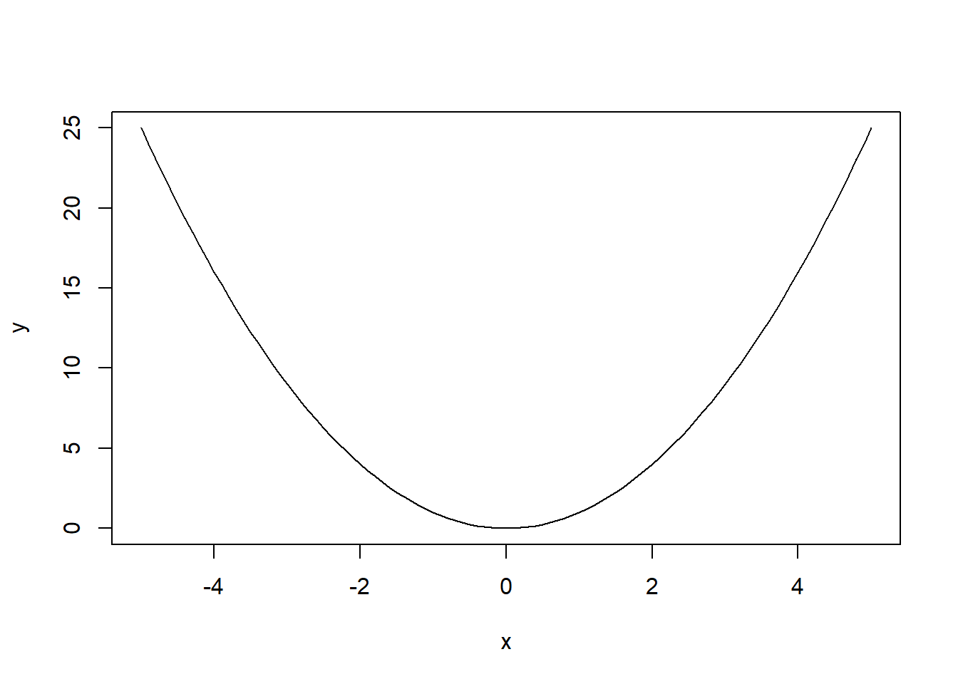

File formats "jpeg" and "png" may be used to produce graphics that can be imported into Word documents, while "pdf" and "postscript" formats into latex documents.

# save graphics as files
dev.copy(jpeg,"quadratic.jpg", quality=95)
dev.off()
dev.copy(pdf,"quadratic.pdf", width=8, height=6)
dev.off()

The help system

R comes with a built-in help system, which may be accessed using the help() function, i.e. help(plot). To search for a specific topic use help.search(). Some of these help outputs can be quite long and you may therefore like to know about the example() command, which makes R work through the examples in the help file. For example, consider the persp() command.

# help
help(persp)
example(persp)

So, what do you think about this initial R tutorial? It can be quite boring at the beginning, but once you overcome the basics the real fun begins!

References

Field, Andy, Zoe Field, and Jeremy Miles. 2012. “Discovering Statistics Using r.”

What is R?

Starting R