
| Well | Sick | Dead | Total | |
|---|---|---|---|---|
| Well | 0.45 | 0.35 | 0.20 | 1 |
| Sick | 0.05 | 0.60 | 0.35 | 1 |
| Dead | 0.00 | 0.00 | 1.00 | 1 |
Markov Models in Economic Evaluations
Quarto
R
Academia
Health Economics
Hello dear readers and welcome to a new post of my blog. Today, I would like to continue the discussion initiated with the last post about modelling in health economic evaluations, particularly with respect to the construction and implementation of decision analytic models or DAMs, such as the Decision Tree Models that were introduced last time. Picking up on this trend, in this post I would like to introduce and talk about Markov Models in economic evaluation, mostly drawing inspiration and references from the book Khan (2015) (Chapter 6) which contains a nice introduction and overview on this topic. As usual warning for the casual reader: in this post I may use some terms that are specific to the health economics literature and field without diving into too many explanations; when this is the case, please bear with me and perhaps make a quick online search (or check my previous posts) to check if anything is unclear to you. For a look at how to implement more complex types of markov models, I recommend checking this nice post, although it is mostly focussed on the implementation of such models in Excel, and heemod package vignette for R.
Markov Models
When the complexity of the modelling task for disease progression increases considerably, e.g. because of many possible mutually exclusive outcomes or the need to repeat the analysis at given time intervals, the use and implementation of decision tree (explored in the previous post) may become quite burdensome. Rather than creating very complex branches and estimate the costs and effects associated with each possible outcome within each branch of the decision tree, it is often more useful to specify the modelling task with respect to the transition of the patients through different (and more limited) health states via Markov Models. More specifically, a Markov model in economic evaluation aims at modelling the transition of patients from one health state to another, and estimate the costs and effects expected to accrue as a result of transitions between health states over a period of time. The period of time over which these transitions are observed (denoted as cycle) may vary depending on the context and the type of disease being modelled, e.g. a week, a month, a year, or even a lifetime.
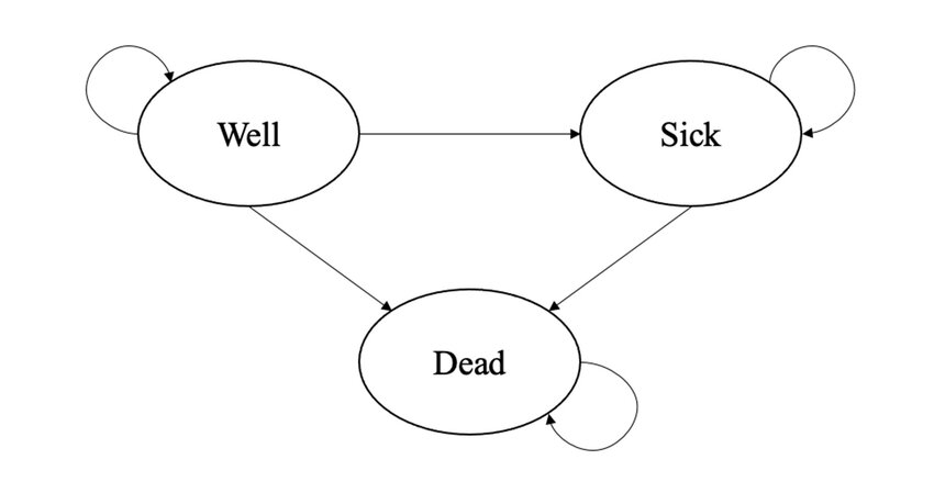
In Markov Models, the probabilities of moving between health states are captured as a matrix of probabilities called a transition matrix, where chance of moving to a different health state depends only on the current health state (and not on health states prior to the current state). This is called the Markov property: \(X_{t+1} = X_t + \varepsilon\), where \(X_{t+1}\) is the health state at time \(t+1\) and is dependent only on the current health state \(X_t\). An example of a simple Markov model is shown in the thumbnail figure of this post and formed by three health states (well, sick, dead) and arrows denoting the direction of the possible transitions between states. Since Markov Models are mostly simulation-based methods, no individual-level data are used to fit the models which are instead based on some aggregated data obtained from the literature or expert elicitation. This also includes the choice for the values of the transition probabilities, whose identification and selection should go through a rigorous process to ensure its reliability and appropriateness.
A simple example
As a demonstrative example, let’s consider the transition matrix shown in Table 1, which displays the assumed transition probabilities for three health states (Well, Sick and Dead) from baseline (rows) to 1 month follow-up (columns), for an hypothetical experimental treatment.
Let’s also assume that patients were randomised to one of two treatments, namely Experimental vs Control, and they were considered to be in either a Well or Sick state. From Table 1, we can see that the proportion of patients who started the hypothetical trial at baseline in a Well state and then remained in the same state after treatment was \(45\%\), very few patients (\(5\%\)) who started the trial in a Sick state improved into a Well state at follow up, and \(60\%\) of patients who were in the Sick state did not change states after starting treatment. In order to compute what the transition matrix will look like after \(1\) month, we need to know the initial probabilities (or the probabilities at baseline), say equal to the first row of Table 1. After \(1\) month of treatment, the transition matrix is updated by multiplying the initial probabilities by the \(3\times3\) transition matrix in Table 1:
tm_update <- matrix(c(0.45,0.05,0,0.35,0.6,0,0.2,0.35,1),3,3)
tm_init <- c(0.45,0.35,0.2)
tm_1m <- tm_init%*%tm_update

tm_1m
[,1] [,2] [,3]
[1,] 0.22 0.3675 0.4125The above \(1\times3\) “matrix” denotes the probabilities in each of the three health states of the model at 1 month after treatment and becomes the initial matrix needed for further calculations. After \(2\) months (second cycle of the process), the updated transition matrix is obtained by multiplying the above matrix again by the \(3 \times 3\) transition matrix in Table 1, and so on. In general, one can compute the proportion of patients for the \(n+1\)-th step in any of these three health states by simply multiplying the updated transition matrix at step \(n\) by the given transition matrix:
\[ M_n = M_{n-1}\times P, \] where \(M_n\) and \(M_{n-1}\) denote the \(1\times 3\) transition matrix at step \(n\) and \(n-1\), while \(P\) denotes the constant \(3\times3\) transition matrix used to update the probabilities at each step. Finally, the last important factor associated with the Markov model is the duration of the interval of time, termed a cycle, set to \(1\) month in the example above. In general, the length of the cycle could be longer or shorter, with shorter cycles needing more computations since they imply a more frequent update of the transition probabilities, i.e. more steps to run.
To continue our example, let’s now consider a more realistic scenario where the transition matrix and initial probabilities are provided for both an experimental group and a control group form an hypothetical trial assessing the cost-effectiveness of the two treatments. The \(3\times3\) transition matrices associated with the two treatments (\(P^{exp},P^{ctr}\)) are shown in Table 2, while the \(1\times3\) matrices of the initial probabilities (\(M^{exp}_0,M^{ctr}_{0}\)) of the two groups are assumed to be equal to the first row of their respective transition matrices.
| Well | Sick | Dead | Total | |
|---|---|---|---|---|
| Well | 0.25 | 0.25 | 0.50 | 1 |
| Sick | 0.10 | 0.45 | 0.45 | 1 |
| Dead | 0.00 | 0.00 | 1.00 | 1 |
We can therefore update the transition matrices of the two treatments over \(5\) cycles, each of \(1\) month, by doing the following
#experimental treatment
tm_exp_update <- matrix(c(0.45,0.05,0,0.35,0.6,0,0.2,0.35,1),3,3)
tm_exp_init <- c(0.45,0.35,0.2)
#update over 5 cycles
tm_exp_1m <- tm_exp_init%*%tm_exp_update
tm_exp_2m <- tm_exp_1m%*%tm_exp_update
tm_exp_3m <- tm_exp_2m%*%tm_exp_update
tm_exp_4m <- tm_exp_3m%*%tm_exp_update
tm_exp_5m <- tm_exp_4m%*%tm_exp_update

#control treatment
tm_ctr_update <- matrix(c(0.25,0.10,0,0.25,0.45,0,0.50,0.45,1),3,3)
tm_ctr_init <- c(0.25,0.25,0.50)
#update over 5 cycles
tm_ctr_1m <- tm_ctr_init%*%tm_ctr_update
tm_ctr_2m <- tm_ctr_1m%*%tm_ctr_update
tm_ctr_3m <- tm_ctr_2m%*%tm_ctr_update
tm_ctr_4m <- tm_ctr_3m%*%tm_ctr_update
tm_ctr_5m <- tm_ctr_4m%*%tm_ctr_update

#experimental TM at the end of 5th cycle
tm_exp_5m
[,1] [,2] [,3]
[1,] 0.02642064 0.1077694 0.86581#control TM at the end of 5th cycle
tm_ctr_5m [,1] [,2] [,3]
[1,] 0.005600547 0.01602453 0.9783749Once the transition probabilities over the desired number of cycles are estimated, further data manipulation can be carried out to estimate the expected costs and effects, which can be included in an additional vector and then multiplied with the elements of the matrices after each cycle to generate the expected total costs and effects. As an example, let’s assume that patients were treated for \(3\) months but followed up for \(12\) months during the trial and that costs were collected from patients files and measured in euros, while effects were collected via self-reported questionnaires (e.g. EQ-5D) and measured via utilities. We need to associate to each health state and treatment in the model a corresponding value for each of the outcomes that we want to measure, i.e. costs and utilities. Thus, we may assume that (monthly) utilities for each health state are \(u^{well}=0.78\), \(u^{sick}=0.40\), and \(u^{dead}=0\), but are constant across treatments. Conversely, we may assume that (monthly) costs are constant across health states but vary between treatment groups, i.e. \(c_{exp}=954\) and \(c^{ctr}=435\). Next, we need to determine the number of cycles of the model. In this case, we will use \(12\) cycles given that we focus over a \(1\) year follow-up, with each cycle being \(1\) month long. Hence, the expected costs and QALYs for each month will be generated and then added up.
The proportion of patients in each of the health states at the start of the model needs to be determined, typically an arbitrary large number, e.g. \(10000\), since the idea is to estimate the cumulative costs and effects over the \(10000\) patients for each group. We can now proceed to calculate the transition matrices and total costs and QALYs associated with both treatment groups over \(12\) months via our Markov Model.
#set up initial values for the model

#initial transition probs by arm
tm_exp_init <- c(0.45,0.35,0.2)
tm_ctr_init <- c(0.25,0.25,0.50)
#transition matrices by arm
tm_exp_update <- matrix(c(0.45,0.05,0,0.35,0.6,0,0.2,0.35,1),3,3)
tm_ctr_update <- matrix(c(0.25,0.10,0,0.25,0.45,0,0.50,0.45,1),3,3)
#utilities by health state
u_well <- 0.78
u_sick <- 0.4
u_dead <- 0
#costs by arm
c_exp <- 954
c_ctr <- 435
#number of cycles
n_cycle <- 12
#initial number of patients in the cohort
n_pat <- 10000

#end of cycle 1 TP
trans_mat_cycle1_exp <- tm_exp_init%*%tm_exp_update
trans_mat_cycle1_ctr <- tm_ctr_init%*%tm_ctr_update
#lists to store TP results by cycle
trans_mat_cycles_exp <- list()
trans_mat_cycles_ctr <- list()


#create function to run the model
mm_sim <- function(tm_exp_init,tm_ctr_init,tm_exp_update,tm_ctr_update,
                   u_well,u_sick,u_dead,c_exp,c_ctr,n_cycle,n_pat){

  res_list <- res_list_exp <- res_list_ctr <- list()
  #set up matrices to contain results from all TP over each cycle by group
  tm_exp <- matrix(NA, nrow = n_cycle+1, ncol = 3)
  colnames(tm_exp) <- c("Well","Sick","Dead")
  tm_ctr <- matrix(NA, nrow = n_cycle+1, ncol = 3)
  colnames(tm_ctr) <- c("Well","Sick","Dead")
  #assign first row to be initial TP
  tm_exp[1,] <- tm_exp_init
  tm_ctr[1,] <- tm_ctr_init
  #loop through cycles and update TM at each cycle
  for(i in 2:c(n_cycle+1)){
    tm_exp[i,] <- tm_exp[i-1,]%*%tm_exp_update
    tm_ctr[i,] <- tm_ctr[i-1,]%*%tm_ctr_update
  }
  #remove intial TP from matrices
  tm_exp <- tm_exp[-1,]
  tm_ctr <- tm_ctr[-1,]
  #using obtained TM to compute number of patients in each health state at each cycle
  npat_cycle_exp <- matrix(NA, nrow = n_cycle+1, ncol = 3)
  colnames(npat_cycle_exp) <- c("Well","Sick","Dead")
  npat_cycle_ctr <- matrix(NA, nrow = n_cycle+1, ncol = 3)
  colnames(npat_cycle_ctr) <- c("Well","Sick","Dead")
  npat_cycle_exp <- tm_exp*n_pat
  npat_cycle_ctr <- tm_ctr*n_pat
  #and number still alive
  nailive_cycle_exp <- as.matrix(rowSums(npat_cycle_exp[,-3]))
  colnames(nailive_cycle_exp) <- "nalive"
  nailive_cycle_ctr <- as.matrix(rowSums(npat_cycle_ctr[,-3]))
  colnames(nailive_cycle_ctr) <- "nalive"
  #use obtained number of patients at each cycle to get the same for costs and QALYs
  costs_cycle_exp <- as.matrix(rowSums(as.matrix(tm_exp*c_exp)[,-3]))
  colnames(costs_cycle_exp) <- "costs"
  costs_cycle_ctr <- as.matrix(rowSums(as.matrix(tm_ctr*c_ctr)[,-3]))
  colnames(costs_cycle_ctr) <- "costs"
  QALY_cycle_exp <- matrix(NA, nrow = n_cycle+1, ncol = 3)
  colnames(QALY_cycle_exp) <- c("Well","Sick","Dead")
  QALY_cycle_ctr <- matrix(NA, nrow = n_cycle+1, ncol = 3)
  colnames(QALY_cycle_ctr) <- c("Well","Sick","Dead")
  u_well_v <- rep(u_well,n_cycle)
  u_sick_v <- rep(u_sick,n_cycle)
  u_dead_v <- rep(u_dead,n_cycle)
  u_M <- cbind(u_well_v,u_sick_v,u_dead_v)
  QALY_cycle_exp <- as.matrix(rowSums(as.matrix(tm_exp*u_M)[,-3]))
  colnames(QALY_cycle_exp) <- c("QALYs")
  QALY_cycle_ctr <- as.matrix(rowSums(as.matrix(tm_ctr*u_M)[,-3]))
  colnames(QALY_cycle_ctr) <- c("QALYs")
  #save output
  res_list_exp[[1]] <- tm_exp
  res_list_exp[[2]] <- npat_cycle_exp
  res_list_exp[[3]] <- nailive_cycle_exp
  res_list_exp[[4]] <- costs_cycle_exp
  res_list_exp[[5]] <- QALY_cycle_exp
  res_list_ctr[[1]] <- tm_ctr
  res_list_ctr[[2]] <- npat_cycle_ctr
  res_list_ctr[[3]] <- nailive_cycle_ctr
  res_list_ctr[[4]] <- costs_cycle_ctr
  res_list_ctr[[5]] <- QALY_cycle_ctr
  names(res_list_exp)<-c("TM","npatients","nalive","costs","QALYs")
  names(res_list_ctr)<-c("TM","npatients","nalive","costs","QALYs")
  res_list[[1]] <- res_list_exp
  res_list[[2]] <- res_list_ctr
  names(res_list)<-c("Experimental","Control")
  return(res_list)
}

#run the function and get the output
mm_res <- mm_sim(tm_exp_init = tm_exp_init, tm_ctr_init = tm_ctr_init, tm_exp_update = tm_exp_update,
       tm_ctr_update = tm_ctr_update, u_well = u_well, u_sick = u_sick, u_dead = u_dead, c_exp = c_exp,
       c_ctr = c_ctr, n_cycle = n_cycle, n_pat = n_pat)
For example, we can extract information regarding the number of patients associated with each health state at each cycle of the model for both intervention groups:
#experimental
mm_res$Experimental$npatients
Well Sick Dead
[1,] 2200.00000 3675.00000 4125.000
[2,] 1173.75000 2975.00000 5851.250
[3,] 676.93750 2195.81250 7127.250
[4,] 414.41250 1554.41562 8031.172
[5,] 264.20641 1077.69375 8658.100
[6,] 172.77757 739.08849 9088.134
[7,] 114.70433 503.92524 9381.370
[8,] 76.81321 342.50166 9580.685
[9,] 51.69103 232.38562 9715.923
[10,] 34.88024 157.52323 9807.597
[11,] 23.57227 106.72203 9869.706
[12,] 15.94362 72.28351 9911.773#control
mm_res$Control$npatients Well Sick Dead
[1,] 875.0000000 1750.000000 7375.000
[2,] 393.7500000 1006.250000 8600.000
[3,] 199.0625000 551.250000 9249.688
[4,] 104.8906250 297.828125 9597.281
[5,] 56.0054687 160.245313 9783.749
[6,] 30.0258984 86.111758 9883.862
[7,] 16.1176504 46.256766 9937.626
[8,] 8.6550892 24.844957 9966.500
[9,] 4.6482680 13.344003 9982.008
[10,] 2.4964673 7.166868 9990.337
[11,] 1.3408037 3.849208 9994.810
[12,] 0.7201217 2.067344 9997.213or the costs and QALYs accrued at each cycle across the alive patients
#experimental
mm_res$Experimental$costs
costs
[1,] 560.475000
[2,] 395.790750
[3,] 274.060350
[4,] 187.826203
[5,] 128.017275
[6,] 86.992022
[7,] 59.017262
[8,] 40.002639
[9,] 27.100912
[10,] 18.355292
[11,] 12.430076
[12,] 8.416869mm_res$Experimental$QALYs QALYs
[1,] 0.318600000
[2,] 0.210552500
[3,] 0.140633625
[4,] 0.094500800
[5,] 0.063715850
[6,] 0.043040190
[7,] 0.029103948
[8,] 0.019691497
[9,] 0.013327325
[10,] 0.009021588
[11,] 0.006107518
[12,] 0.004134943#control
mm_res$Control$costs costs
[1,] 114.1875000
[2,] 60.9000000
[3,] 32.6385937
[4,] 17.5182656
[5,] 9.4069090
[6,] 5.0519880
[7,] 2.7132871
[8,] 1.4572520
[9,] 0.7826638
[10,] 0.4203551
[11,] 0.2257655
[12,] 0.1212548mm_res$Control$QALYs QALYs
[1,] 0.1382500000
[2,] 0.0709625000
[3,] 0.0375768750
[4,] 0.0200945938
[5,] 0.0107782391
[6,] 0.0057864904
[7,] 0.0031074474
[8,] 0.0016688952
[9,] 0.0008963250
[10,] 0.0004813992
[11,] 0.0002585510
[12,] 0.0001388633from which an estimate of the mean costs and QALYs (and the group differences) over the \(12\) months period (without discounting) can be obtained by taking the sum across these accrued expected values at each cycle
#experimental
mu_c_exp <- sum(mm_res$Experimental$costs)
mu_e_exp <- sum(mm_res$Experimental$QALYs)

#control
mu_c_ctr <- sum(mm_res$Control$costs)
mu_e_ctr <- sum(mm_res$Control$QALYs)

mu_c_diff <- mu_c_exp-mu_c_ctr
mu_e_diff <- mu_e_exp-mu_e_ctr
and from this an estimate of the ICER can be obtained:
\[ \text{ICER} = \frac{1798.4846494 - 245.4238347}{0.9524298-0.2900002} =\frac{1553.0608148}{0.6624296} = 2344.49 \]
I hope you enjoyed today’s topic as it was quite interesting, at least for me. I always want to learn more about this stuff and rarely have the time do so. By going through the coding, I think things become much easier to understand, especially when these types of models can be quite complex and difficult to grasp by just reading it on a paper. Probably next time I will dive into the uncertainty assessment for these models, which at the moment I neglected due to time constraints. Well, I hope to see you back on my next post to learn how to do that as well (if you are interested).
References
Khan, Iftekhar. 2015. Design & Analysis of Clinical Trials for Economic Evaluation & Reimbursement: An Applied Approach Using SAS & STATA. CRC Press.