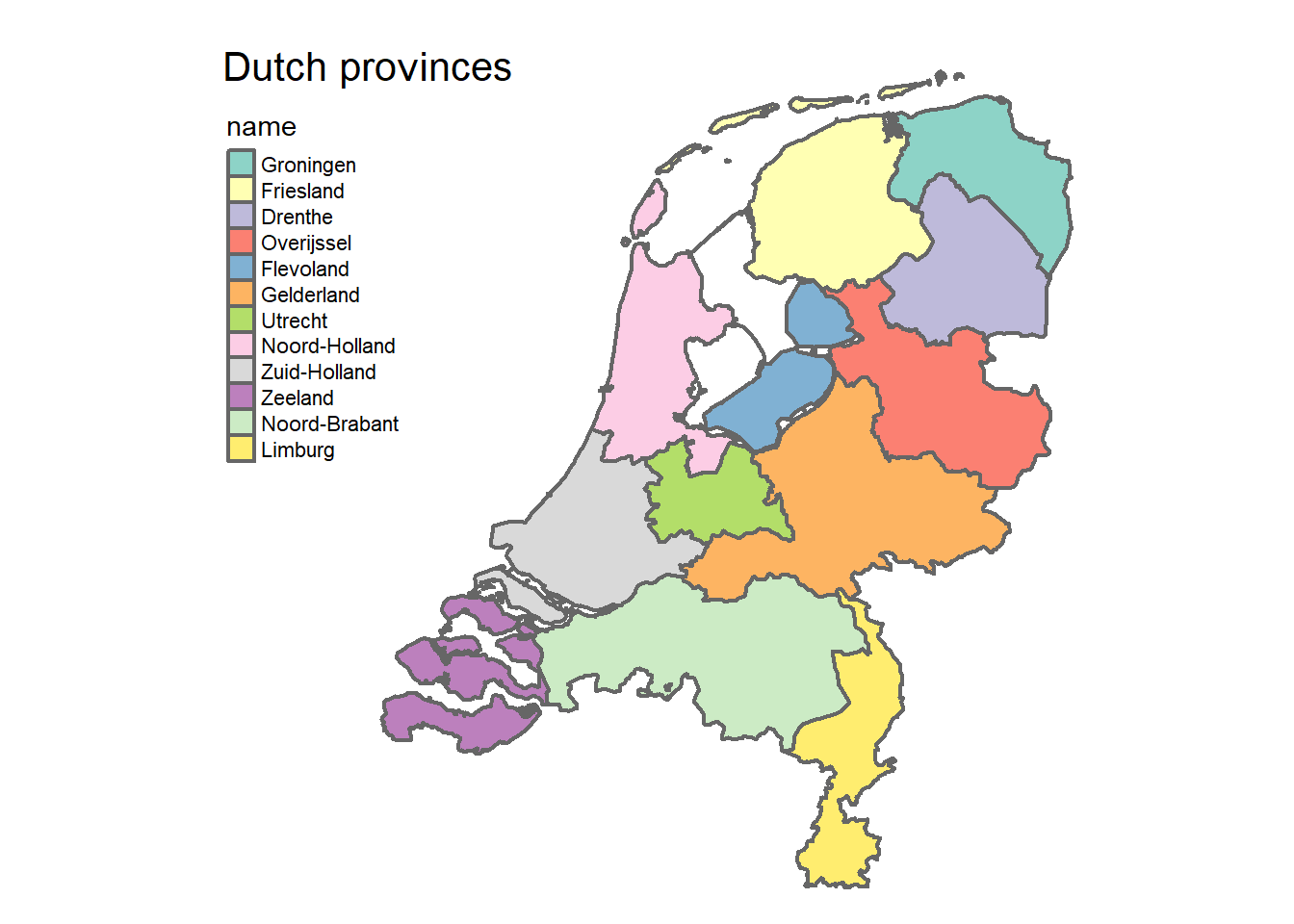
library(tmap)
tmap_mode("plot")
data(NLD_prov)
tm_shape(NLD_prov) +
  tm_borders(lwd=2) +
  tm_fill("name") +
  tm_format("NLD", title="Dutch provinces", bg.color="white")
September 14, 2024
 Hello dear readers, I hope everything is well with you and welcome back for another post on my site. Today I would like to continue the little exercise I started last time where I played a bit using some Dutch data related to the different provinces of the country to make some comparisons between them. Again, I apologise to my readers who are looking forward to some more health economics topic, but I really want to continue the previous topic with some additional fun examples.
What I am focussing today is still about using some Dutch-province level data, this time taken directly from the CBS website and related to the average number of travels per person per year. My basic idea is very simple. Which province has the largest average number of travels per year? and can we also identify some temporal trend? in order to answer this question I have taken from the above link information about the average number of travels per person per year for each of the \(12\) provinces of the Netherlands over a period of \(6\) years, between 2018 and 2023.
As usual, let’s start by drawing a map of the country divided into provinces:

Next, let’s download the CBS data we are interested as a .csv file, import it into R and let’s explore the data.
NLD_prov_travel <- read.csv("per_person__travel_modes__travel_purpose_16092024_155133.csv", header = T, sep = ";")

#create a subset of the dataset and rename the variables
NLD_prov_travel <- NLD_prov_travel[,5:7]
names(NLD_prov_travel) <- c("Province","Year","Travels")

#let's extract the travel data for all provinces for 1 year first, say 2023
NLD_prov_travel_2023 <- NLD_prov_travel[NLD_prov_travel$Year==2023,]

#see the data
NLD_prov_travel_2023
Province Year Travels
6 Groningen (PV) 2023 994
12 Fryslân (PV) 2023 995
18 Drenthe (PV) 2023 988
24 Overijssel (PV) 2023 1054
30 Flevoland (PV) 2023 936
36 Gelderland (PV) 2023 1036
42 Utrecht (PV) 2023 1029
48 Noord-Holland (PV) 2023 954
54 Zuid-Holland (PV) 2023 945
60 Zeeland (PV) 2023 974
66 Noord-Brabant (PV) 2023 1023
72 Limburg (PV) 2023 1011We can see that in 2023 it appears that Overijssel, Gelderland, Utrecht, and Noord-Brabant were the provinces associated with most average number of travels per person (above \(1020\) travels). It could interesting to get some information about how the number of travels has changed over time for each province. To achieve this we can try to compute some summary statistics:
#load package
library(data.table)
#create custom summary function
my.summary <- function(x, na.rm=TRUE){list(n= length(x),
                                  Mean=mean(x),
                                  SD=sd(x),
                                  Median=median(x),
                                  Min=min(x),
                                  Max=max(x))}
#summarise data
sum_data_travel <- setDT(NLD_prov_travel)[, unlist(lapply(.SD, my.summary),recursive=FALSE), Province]

#extract and display relevant data
sum_data_travel.dt <- sum_data_travel[,c(1,8:13)]
sum_data_travel.dt
Province Travels.n Travels.Mean Travels.SD Travels.Median
<char> <int> <num> <num> <num>
1: Groningen (PV) 6 941.3333 72.39797 959.5
2: Fryslân (PV) 6 960.5000 39.53606 972.0
3: Drenthe (PV) 6 976.1667 55.27537 985.0
4: Overijssel (PV) 6 1002.1667 67.49049 1034.0
5: Flevoland (PV) 6 905.0000 58.61058 920.5
6: Gelderland (PV) 6 999.0000 59.04574 1026.0
7: Utrecht (PV) 6 992.8333 65.26689 1023.5
8: Noord-Holland (PV) 6 930.1667 65.12885 950.5
9: Zuid-Holland (PV) 6 923.0000 64.91225 942.5
10: Zeeland (PV) 6 962.0000 55.20507 979.0
11: Noord-Brabant (PV) 6 983.0000 49.52979 1005.0
12: Limburg (PV) 6 963.1667 56.86973 985.5
Travels.Min Travels.Max
<int> <int>
1: 831 1024
2: 908 998
3: 880 1028
4: 886 1054
5: 820 980
6: 905 1046
7: 888 1056
8: 820 1006
9: 814 989
10: 858 1015
11: 904 1023
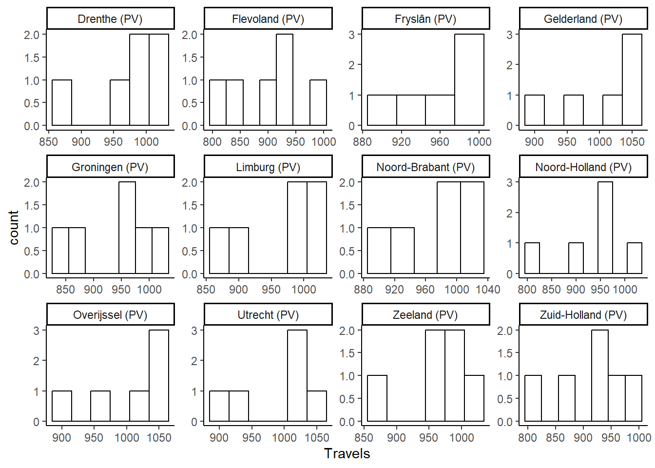
12: 872 1011Creating summary statistics per Province over a period of 6 years (2018-2023), we can see that on average Overijssel still places at the top with a mean number of travels per person of \(1002\), followed by Gelderland (\(999\)) and Utrecht (\(992\)), while all other Provinces seem to fall a bit behind with very similar values between \(900\) and \(976\). However, we also notice that, for some Provinces, median values are a bit different from means (typically higher), with also some minimum and maximum values that can be quite extreme in some cases. So, let’s have a look at the shape of the data distribution. For example, we may plot via histograms the travel data by Province over the 6-year period considered.

Although 6 data points per Province is not a lot to look at, we can notice that for some Provinces the distribution of the number of travels is skewed, therefore suggesting how the mean perhaps is not a good indicator for these data.
What at this point if we want to try and make a prediction of what the number of travels would be for each Province in 2024? and what about the expected number of travels over the 6 year period across all Provinces? Well, for that we need some inferential statistics! For example, taking into account the time dependence of the 6 observations per Province, let’s try to fit a linear mixed effects model including a random error term to capture the clustering nature of the data at the level of the Provinces:
\[ \text{Travel}_{ij} = \beta_0 + \beta_1 \times \text{Year} + \omega_j + \varepsilon_{ij} \]
where: \(\text{Travel}_{ij}\) refers to the number of travels per person for Province \(i\) in Year \(j\), while \(\beta_0\) is the intercept, \(\beta_1\) is the year regression coefficient, \(\varepsilon_{ij}\) and \(\omega_j\) are the random error term and the Province-specific random effect term.
#load package
library(lme4)
fm <- lmer(Travels ~ Year + (1 | Province), data = NLD_prov_travel)
#define new data for prediction
newdata <- expand.grid(
  Year = c(2024),
  Province = unique(NLD_prov_travel$Province)
)
#predict
fm_pred <- predict(fm, newdata = newdata)
names(fm_pred) <- unique(NLD_prov_travel$Province)

#look at predictions
fm_pred
Groningen (PV) Fryslân (PV) Drenthe (PV) Overijssel (PV)
948.6030 955.9821 962.0137 972.0237
Flevoland (PV) Gelderland (PV) Utrecht (PV) Noord-Holland (PV)
934.6147 970.8045 968.4304 944.3038
Zuid-Holland (PV) Zeeland (PV) Noord-Brabant (PV) Limburg (PV)
941.5447 956.5596 964.6445 957.0087 We can see that, according to the model predictions Overijssel still is associated with the largest number of travels even in 2024, followed by Gelderland and Utrecht, although the difference now seems a little bit smaller compared to what observed from the descriptive analysis of the data. Finally, we can also try to obtain an estimate of the average number of travels across Years and Provinces. This can be done, if we consider Year as a continuous variable, by setting its value equal to the average across the years considered (\(\bar{\text{Year}}=\text{E}[\text{Year}]_i\), for \(i=,2018,2019,\ldots,2023\)), generate the predictions by Province, and then take the expectation across them.
[1] 961.5278So, based on the model and data, we would expect an average number of travels per person across Provinces between 2018-2023 of about 961.53.
I hope you enjoyed this little exercise as much as I did. It is a nice distraction from the usual work I do and a bit of fesh air. But no worries, I will soon come back to talk more about health economics and Bayesian statstics!